熊貓分發
This article is a continuation of a previous article which kick-started the journey to learning Python for data analysis. You can check out the previous article here: Pandas for Newbies: An Introduction Part I.
本文是上一篇文章的延續,該文章開始了學習Python進行數據分析的旅程。 您可以在此處查看上一篇文章: 新手熊貓:簡介第一部分 。
For those just starting out in data science, the Python programming language is a pre-requisite to learning data science so if you aren’t familiar with Python go make yourself familiar and then come back here to start on Pandas.
對于剛接觸數據科學的人來說,Python編程語言是學習數據科學的先決條件,因此,如果您不熟悉Python,請先熟悉一下,然后再回到這里開始學習Pandas。
You can start learning Python with a series of articles I just started called Minimal Python Required for Data Science.
您可以從我剛剛開始的一系列文章開始學習Python,這些文章稱為“數據科學所需的最小Python” 。
As a reminder, what I’m doing here is a brief tour of just some of the things you can do with Pandas. It’s the deep-dive before the actual deep-dive.
提醒一下,我在這里所做的只是對熊貓可以做的一些事情的簡要介紹。 這是真正的深潛之前的深潛。
Both the data and the inspiration for this series comes from Ted Petrou’s excellent courses on Dunder Data.
數據和本系列的靈感都來自Ted Petrou的Dunder Data精品課程。
先決條件 (Prerequisites)
- Python Python
- pandas 大熊貓
- Jupyter 朱皮特
You’ll be ready to begin once you have these three things in order.
將這三件事整理好后,您就可以準備開始。
聚合 (Aggregation)
We left off last time with the pandas query method as an alternative to regular filtering via boolean conditional logic. While it does have its limits, the query is a much more readable method.
上一次我們沒有使用pandas query方法,而是通過布爾條件邏輯進行常規過濾的替代方法。 盡管確實有其限制,但query是一種更具可讀性的方法。
Today we continue with aggregation which is the act of summarizing data with a single number. Examples include sum, mean, median, min and max.
今天,我們繼續進行匯總,這是用單個數字匯總數據的操作。 示例包括總和,均值,中位數,最小值和最大值。
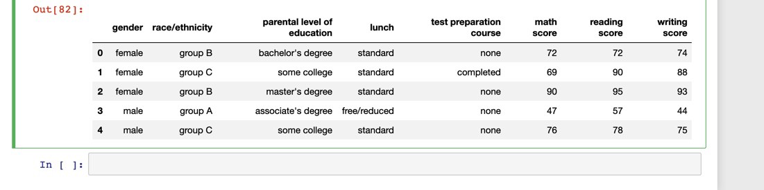
Let’s try this on different dataset.
讓我們在不同的數據集上嘗試一下。
Get the mean by calling the mean method.
通過調用均值方法獲得均值。
students.mean()math score       66.089
reading score    69.169
writing score    68.054
dtype: float64
User the axis parameter to calculate the sum of all the scores (math, reading, and writing) across rows:
使用axis參數來計算各行中所有分數的總和(數學,閱讀和寫作):
scores = students[['math score', 'reading score', 'writing score']]scores.sum(axis=1).head(3)0    218
1    247
2    278
dtype: int64
非匯總方法 (Non-aggregating methods)
Perform calculations on the data that do not necessarily aggregate the data. I.E. the round method:
對不一定要匯總數據的數據執行計算。 IE的round方法:
scores.round(-1).head(3)math score reading score writing score0 70 70 701 70 90 902 90 100 90組內匯總 (Aggregating within groups)
Let’s get the frequency of unique values in a single column.
讓我們在單個列中獲得唯一值的頻率。
students['parental level of education'].value_counts()some college 226
associate's degree 222
high school 196
some high school 179
bachelor's degree 118
master's degree 59
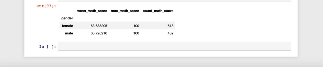
Name: parental level of education, dtype: int64Use the groupby method to create a group and then apply and aggregation. Here we get the mean math scores for each gender:
使用groupby方法創建一個組,然后應用和聚合。 在這里,我們獲得了每種性別的平均數學成績:
students.groupby('gender').agg(
    mean_math_score=('math score', 'mean')
)mean_math_scoregenderfemale        63.633205male          68.728216
多重聚合 (Multiple aggregation)
Here we do multiple aggregations at the same time.
在這里,我們同時進行多個聚合。
students.groupby('gender').agg(
    mean_math_score=('math score', 'mean'),
    max_math_score=('math score', 'max'),
    count_math_score=('math score', 'count')
)
We can create groups from more than one column.
我們可以從多個列中創建組。
students.groupby(['gender', 'test preparation course']).agg(
    mean_math_score=('math score', 'mean'),
    max_math_score=('math score', 'max'),
    count_math_score=('math score', 'count')
)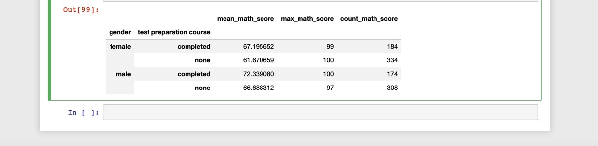
It looks like students who prepped for test for both sexes scored higher than those who didn’t.
看來為兩性做準備的學生的得分都比那些沒有參加過測試的學生要高。
數據透視表 (Pivot Table)
A better way to present information to consumers of information would be to use the pivot_table function which does the same thing as groupby but makes use of one of the grouping columns as the new columns.
將信息呈現給信息消費者的一種更好的方法是使用pivot_table函數,該函數與groupby相同,但是將分組列之一用作新列。
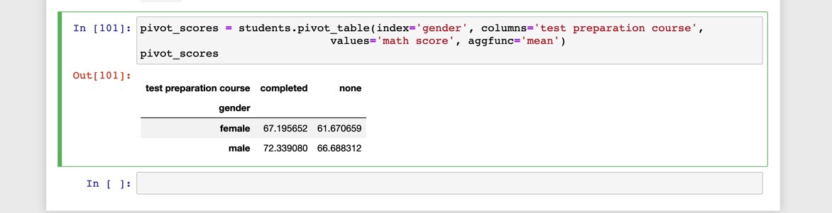
Again, it’s the same information presented in a more readable and intuitive format.
同樣,它是以更易讀和直觀的格式呈現的相同信息。
數據整理 (Data Wrangling)
Let’s bring a new dataset to examine datasets with missing values
讓我們帶來一個新的數據集來檢查缺少值的數據集
providing the na_values argument will mark the NULL values in a dataset as NaN (Not a Number).
提供na_values參數會將數據集中的NULL值標記為NaN(非數字)。
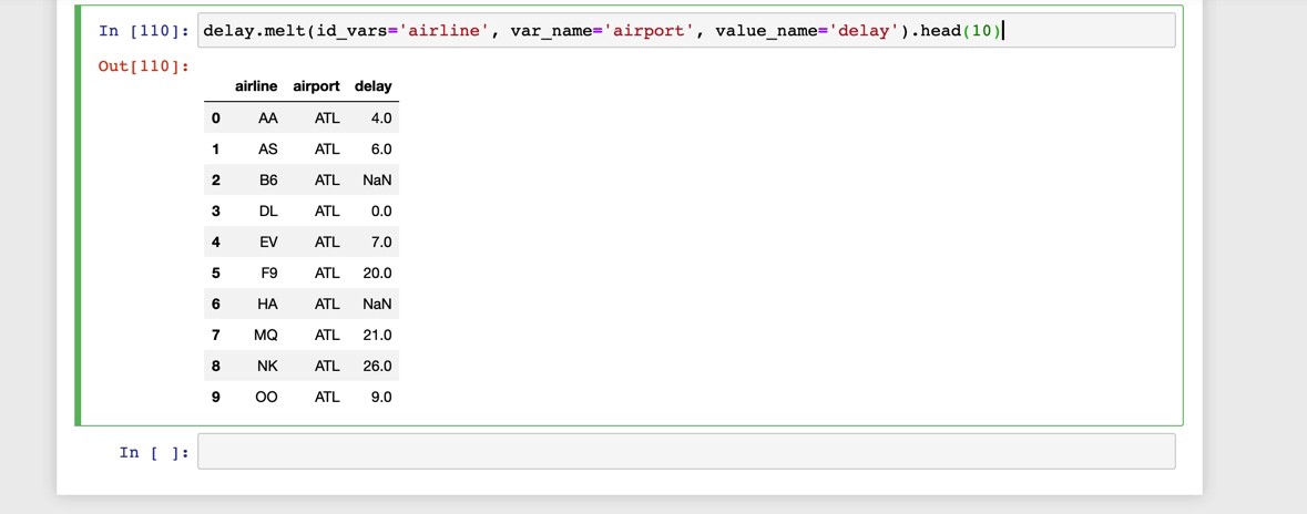
You might also be confronted with a dataset where all the columns should all be part of one column.
您可能還會遇到一個數據集,其中所有列都應該都屬于一個列。
We can use the melt method to stack columns one after another.
我們可以使用melt法將一列又一列堆疊。
合并數據集 (Merging Datasets)
Knowing a little SQL will come in handy when studying this part of the pandas library.
在學習pandas庫的這一部分時,了解一點SQL會很方便。
There are multiple ways to join data in pandas, but the one method you should definitely get comfortable with is the merge method which connects rows in DataFrames based on one or more keys. It’s basically an implementation of SQL JOINS.
在熊貓中聯接數據有多種方法,但是您絕對應該習慣的一種方法是merge方法,該方法基于一個或多個鍵連接DataFrames中的行。 它基本上是SQL JOINS的實現。
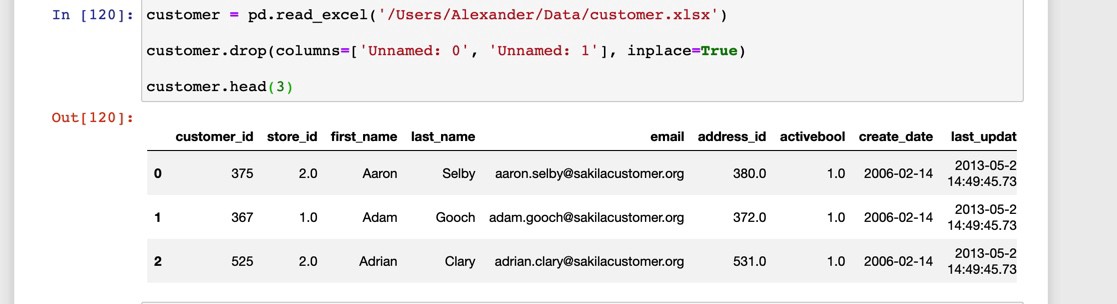
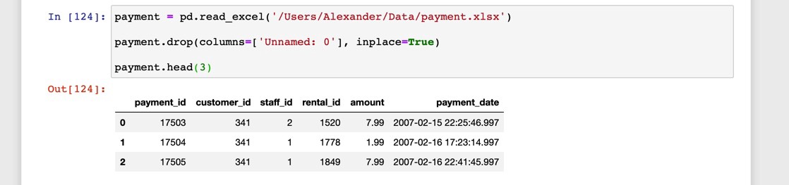
Let’s say I had the following data from a movie rental database:
假設我從電影租借數據庫中獲得了以下數據:
To perform an “INNER” join using merge :
要使用merge執行“ INNER” merge :
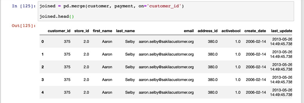
The SQL (PostgreSQL) equivalent would be something like:
等效SQL(PostgreSQL)如下所示:
SELECT * FROM customer
INNER JOIN payment
ON payment.customer_id = customer.customer_id
ORDER BY customer.first_name ASC
LIMIT 5;
時間序列分析 (Time Series Analysis)
The name pandas is actually derived from Panel Data Analysis which combines cross-sectional data with time-series used most widely in medical research and economics.
熊貓這個名字實際上是來自面板數據分析,它結合了橫截面數據和在醫學研究和經濟學中使用最廣泛的時間序列。
Let’s say I had the following data where I knew it was time-series data, but without a DatetimeIndex specifying it as a time-series:
假設我在知道它是時間序列數據的地方有以下數據,但是沒有DatetimeIndex將其指定為時間序列:
p a0 0.749 28.961 1.093 67.812 0.920 55.153 0.960 78.624 0.912 60.15I can simply set the index as a DatetimeIndex with:
我可以簡單地將索引設置為DatetimeIndex :
Which results in:
結果是:
p a1986-12-31 0.749 28.961987-12-31 1.093 67.811988-12-31 0.920 55.151989-12-31 0.960 78.621990-12-31 0.912 60.151991-12-31 1.054 45.541992-12-31 1.079 33.621993-12-31 1.525 44.581994-12-31 1.310 41.94Here we have a dataset where p is the dependent variable and a is the independent variable. Before running an econometric model called AR(1) we’d have to lag the dependent variable to deal with autocorrelation which we could do using:
在這里,我們有一個數據集,其中p是因變量,而a是自變量。 在運行稱為AR(1)的計量經濟學模型之前,我們必須將因變量滯后以處理自相關,我們可以使用以下方法進行處理:
p a p_lagged1986-12-31 0.749 28.96 NaN1987-12-31 1.093 67.81 0.7491988-12-31 0.920 55.15 1.0931989-12-31 0.960 78.62 0.9201990-12-31 0.912 60.15 0.960可視化 (Visualization)
The combination of matplotlib and pandas allows us to make rudimentary simple plots in the blink of an eye:
matplotlib和pandas的組合使我們能夠在眨眼間做出基本的簡單圖:
# Using the previous datasetbangla.plot();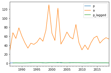
pivot_scores.plot(kind='bar');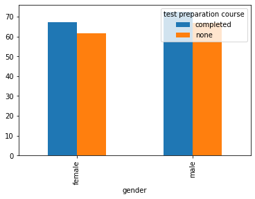
That concludes our brief bus tour of the pandas toolbox for data analysis. There’s a lot more that we’ll dive into for my next series of articles. So stay tuned!
到此為止,我們簡要介紹了熊貓工具箱進行數據分析的過程。 在我的下一系列文章中,我們將涉及更多內容。 敬請期待!
我做的事 (What I do)
I help people find mentors, code in Python, and write about life. If you’re thinking about switching careers into the tech industry or just want to talk you can sign up for my Slack Channel via VegasBlu.
我幫助人們找到導師,用Python編寫代碼,并撰寫有關生活的文章。 如果您正在考慮將職業轉向科技行業,或者只是想談談,可以通過VegasBlu注冊我的Slack頻道。
翻譯自: https://towardsdatascience.com/pandas-for-newbies-an-introduction-part-ii-9f69a045dd95
熊貓分發
本文來自互聯網用戶投稿,該文觀點僅代表作者本人,不代表本站立場。本站僅提供信息存儲空間服務,不擁有所有權,不承擔相關法律責任。 如若轉載,請注明出處:http://www.pswp.cn/news/389155.shtml 繁體地址,請注明出處:http://hk.pswp.cn/news/389155.shtml 英文地址,請注明出處:http://en.pswp.cn/news/389155.shtml
如若內容造成侵權/違法違規/事實不符,請聯系多彩編程網進行投訴反饋email:809451989@qq.com,一經查實,立即刪除!相關文章

淺析微信支付:申請退款、退款回調接口、查詢退款
)
view工作原理-計算視圖大小的過程(onMeasure)
![[轉載]使用.net 2003中的ngen.exe編譯.net程序](http://pic.xiahunao.cn/[轉載]使用.net 2003中的ngen.exe編譯.net程序)
[轉載]使用.net 2003中的ngen.exe編譯.net程序

基于Redis實現分布式鎖實戰

數據分析 績效_如何在績效改善中使用數據分析


您一直在尋找5+個簡單的一線工具來提升Python可視化效果

用C#編寫的代碼經C#編譯器后,并非生成本地代碼而是生成托管代碼

figma 安裝插件_彩色濾光片Figma插件,用于色盲


產品觀念:更好的捕鼠器_故事很重要:為什么您需要成為更好的講故事的人

7月15號day7總結


設計師的10種范式轉變
)
面向Tableau開發人員的Python簡要介紹(第2部分)

GAC中的所有的Assembly都會存放在系統目錄%winroot%/assembly下面
 Mysq慢查詢日志)
Mysql(三) Mysq慢查詢日志

繪制基礎知識-canvas paint
