Most traders use Bollinger Bands. However, price is not normally distributed. That’s why only 42% of prices will close within one standard deviation. Please go ahead and read this article. However, I have some good news.

大多數交易者使用布林帶。 但是，價格不是正態分布的。 這就是為什么只有42％的價格會在一個標準偏差之內收盤的原因。 請繼續閱讀本文 。 但是，我有一些好消息。

Price is not normally distributed. Returns are!

價格不是正態分布。 退貨都是！

Yes price is not normally distributed. Because price is nothing but sum of returns. And returns are normally distributed. So let’s jump in coding and hopefully you will have an “Aha!” moment.

是的，價格不是正態分布。 因為價格不過是回報之和。 收益是正態分布的。 因此，讓我們開始編碼，希望您會得到一個“ 啊哈 ！” 時刻。

I’m going to use EURUSD daily chart in my sample. However, it’s going to work with all assets and all timeframes.

我將在示例中使用EURUSD每日圖表。 但是，它將適用于所有資產和所有時間范圍。

Add required libraries

添加所需的庫

# we only need these 3 libraries
import pandas as pd
import numpy as np
import matplotlib.pyplot as plt

Not let’s write the code to load our time-series dataset

不讓我們編寫代碼來加載時間序列數據集

def load_file(f):
    fixprice = lambda x: float(x.replace(',', '.'))
    df = pd.read_csv(f)
    if "Gmt time" in df.columns:
        df['Date'] = pd.to_datetime(df['Gmt time'], format="%d.%m.%Y %H:%M:%S.%f")
    elif "time" in df.columns:
        df['Date'] = pd.to_datetime(df['time'], unit="s")
        df['Date'] = df['Date'] + np.timedelta64(3 * 60, "m")
        df[['Date', 'Open', 'High', 'Low', 'Close']] = df[['Date', 'open', 'high', 'low', 'close']]
        df = df[['Date', 'Open', 'High', 'Low', 'Close']]
    elif "Tarih" in df.columns:
        df['Date'] = pd.to_datetime(df['Tarih'], format="%d.%m.%Y")
        df['Open'] = df['A??l??'].apply(fixprice)
        df['High'] = df['Yüksek'].apply(fixprice)
        df['Low'] = df['Dü?ük'].apply(fixprice)
        df['Close'] = df['?imdi'].apply(fixprice)
    else:
        df["Date"] = pd.to_datetime(df["Date"])
    # we need to shift or we will have lookahead bias in code
    df["Returns"] = (df["Close"].shift(1) - df["Close"].shift(2)) / df["Close"].shift(2)
    return df

Now if you look at the code, I have added a column “Returns” and it’s shifted. We don’t want our indicator to repaint and i don’t want to have lookahead bias. I am basically calculating the change from yesterday’s close to today’s close and shifting.

現在，如果您看一下代碼，我添加了“ Returns”列，它已轉移。 我們不希望我們的指標重新粉刷，我也不想有前瞻性偏見。 我基本上是在計算從昨天的收盤價到今天的收盤價的變化。

Load your dataset and plot histogram of Returns

加載數據集并繪制退貨的直方圖

sym = "EURUSD"
period = "1d"
fl = "./{YOUR_PATH}/{} {}.csv".format(period, sym)
df = load_file(fl)
df["Returns"].hist(bins=1000, grid=False)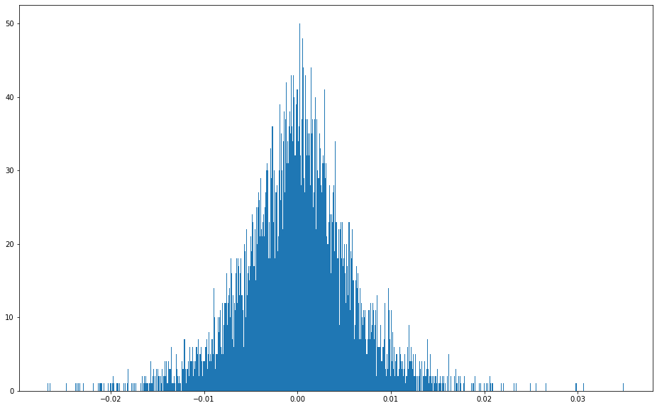

Perfect bell shape curve. Now we know that we can get some real probabilities right? Empirical Rule (a.k.a. 68–95–99.7 rule) states that 68% of data will fall within one standard deviation, 95% of data will fall within two standard deviation and 99.7% of data will fall within three standard deviation. Ok let’s write the code to calculate it for us.

完美的鐘形曲線。 現在我們知道可以得到一些真實的概率了嗎？ 經驗法則 (也稱為68–95–99.7規則)指出，68％的數據將落在一個標準偏差內，95％的數據將落在兩個標準偏差內，而99.7％的數據將落在三個標準偏差內。 好的，讓我們編寫代碼為我們計算一下。

def add_momentum(df, lb=20, std=2):
    df["MA"] = df["Returns"].rolling(lb).mean()
    df["STD"] = df["Returns"].rolling(lb).std()
    df["OVB"] = df["Close"].shift(1) * (1 + (df["MA"] + df["STD"] * std))
    df["OVS"] = df["Close"].shift(1) * (1 + (df["MA"] - df["STD"] * std))
    return df

Now as we already have previous Bar’s close, it’s easy and safe to use and calculate the standard deviation. Also it’s easy for us to have overbought and oversold levels in advance. And they will stay there from the beginning of the current period. I also want to be sure if my data going to follow the empirical rule. So i want to get the statistics. Let’s code that block as well.

現在，由于我們已經關閉了先前的Bar，因此可以輕松安全地使用和計算標準偏差。 同樣，我們很容易提前超買和超賣。 他們將從當前階段開始一直呆在那里。 我還想確定我的數據是否遵循經驗法則。 所以我想獲得統計數據。 讓我們也對該塊進行編碼。

def stats(df):
    total = len(df)
    ins1 = df[(df["Close"] > df["OVS"]) & (df["Close"] < df["OVB"])]
    ins2 = df[(df["Close"] > df["OVS"])]
    ins3 = df[(df["Close"] < df["OVB"])]
    il1 = len(ins1)
    il2 = len(ins2)
    il3 = len(ins3)
    r1 = np.round(il1 / total * 100, 2)
    r2 = np.round(il2 / total * 100, 2)
    r3 = np.round(il3 / total * 100, 2)
    return r1, r2, r3

Now let’s call these function…

現在讓我們稱這些功能為…

df = add_momentum(df, lb=20, std=1)
stats(df)

Output is (67.36, 83.3, 83.77). So close price falls 67.36% within one standard deviation. Closing price is above OVS with 83.3% and below OVB with 83.77%. Amazing results… Now time to plot our bands to see how they look in the chart.

輸出為(67.36、83.3、83.77)。 因此，收盤價在一個標準偏差之內下跌67.36％。 收盤價高于OVS，為83.3％，低于OVB，為83.77％。 驚人的結果...現在該繪制我們的樂隊，看看它們在圖表中的樣子。

I love candles. So let’s code it in a quick and dirty way and plot how our levels look.

我愛蠟燭。 因此，讓我們以一種快速而骯臟的方式對其進行編碼，并繪制出關卡的外觀。

def plot_candles(df, l=0):
    """
        Plots candles
        l: plot last n candles. If set zero, draw all
    """
    db = df.copy()
    if l > 0:
        db = db[-l:]
    db = db.reset_index(drop=True).reset_index()
    db["Up"] = db["Close"] > db["Open"]
    db["Bottom"] = np.where(db["Up"], db["Open"], db["Close"])
    db["Bar"] = db["High"] - db["Low"]
    db["Body"] = abs(db["Close"] - db["Open"])
    db["Color"] = np.where(db["Up"], "g", "r")
    fig, ax = plt.subplots(1, 1, figsize=(16, 9))
    ax.yaxis.tick_right()
    ax.bar(db["index"], bottom=db["Low"], height=db["Bar"], width=0.25, color="#000000")
    ax.bar(db["index"], bottom=db["Bottom"], height=db["Body"], width=0.5, color=db["Color"])
    ax.plot(db["OVB"], color="r", linewidth=0.25)
    ax.plot(db["OVS"], color="r", linewidth=0.25)
    plt.show()

I want to see last 100 candles. Now let’s call this function

我想看最后100支蠟燭。 現在我們叫這個功能

plot_candles(df, l=100)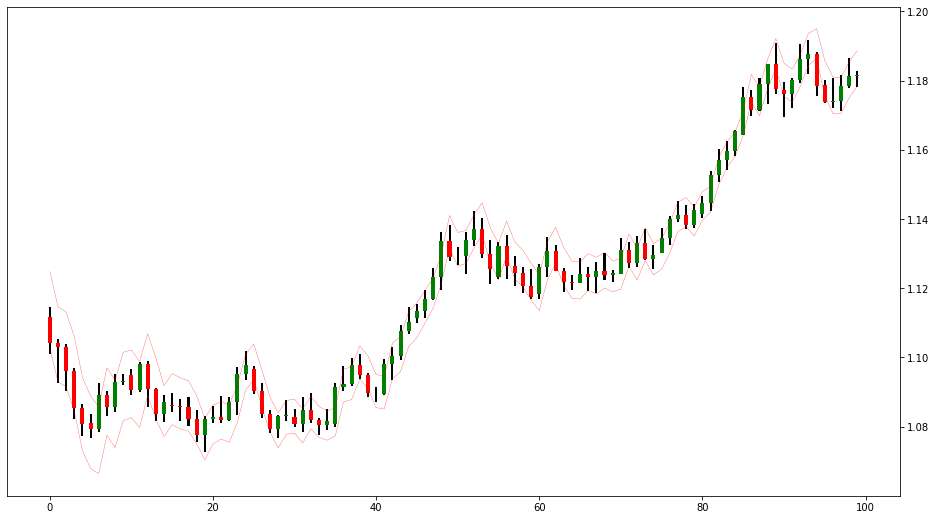

接下來做什么？ (What to do next?)

Well to be honest, if i would be making money using this strategy, i wouldn’t share it here with you (no offense). I wouldn’t even sell it. However, you can use your own imagination and add some strategies on this. You can thank me later if you decide to use this code and make money. I will send you my IBAN later :)

老實說，如果我要使用這種策略來賺錢，我不會在這里與您分享(無罪)。 我什至不賣。 但是，您可以發揮自己的想象力，并為此添加一些策略。 如果您決定使用此代碼并賺錢，稍后可以感謝我。 稍后我將把您的IBAN發送給您：)

Disclaimer

免責聲明

I’m not a professional financial advisor. This article and codes, shared for educational purposes only and not financial advice. You are responsible your own losses or wins.

我不是專業的財務顧問。 本文和代碼僅用于教育目的，不用于財務建議。 您應對自己的損失或勝利負責。

The whole code of this article can be found on this repository:

可以在此存儲庫中找到本文的完整代碼：

Ah also; remember to follow me on the following social channels:

也啊 記得在以下社交渠道關注我：

MediumTwitterTradingViewYouTube!

中級 Twitter TradingViewYouTube ！

Until next time; stay safe, trade safe!!!

直到下一次; 保持安全，交易安全！！！

Atilla Yurtseven

阿蒂拉·尤爾特斯文(Atilla Yurtseven)