高斯分布及其主要特征： (Gaussian Distribution and its key characteristics:)

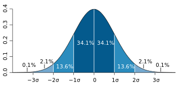
• Gaussian distribution is a continuous probability distribution with symmetrical sides around its center.
  高斯分布是連續概率分布，其中心周圍具有對稱邊。
• Its mean, median and mode are equal.
  其均值，中位數和眾數相等。
• Its shape looks like below with most of the data points clustered around the mean with asymptotic tails.
  它的形狀如下圖所示，大多數數據點均以漸近尾部聚類在均值周圍。

Interpretation:

解釋：

• ~68% of the values drawn from normal distribution lie within 1𝜎
  從正態分布得出的值的約68％位于1𝜎之內
• ~95% of the values drawn from normal distribution lie within 2𝜎
  從正態分布得出的值的約95％位于2𝜎之內
• ~99.7% of the values drawn from normal distribution lie within 3𝜎
  從正態分布得出的值的約99.7％位于3𝜎之內

我們在哪里找到高斯分布的存在？ (Where do we find the existence of Gaussian distribution?)

ML practitioners or not, almost all of us have heard of this most popular form of distribution somewhere or the other. Everywhere we look around us, majority of the processes follow approximate Gaussian form, for e.g. age, height, IQ, memory, etc.

不管是否有ML從業者，我們幾乎所有人都聽說過這種最流行的發行形式。 我們環顧四周的任何地方，大多數過程都遵循近似的高斯形式，例如年齡，身高，智商，記憶力等。

On a lighter note, there is one well-known example of Gaussian lurking around all of us i.e. ‘bell curve’ during appraisal time 😊

輕松地說，有一個眾所周知的例子，高斯潛伏在我們所有人周圍，即在評估期間出現“鐘形曲線”😊

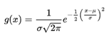
Yes, Gaussian distribution resonates with bell curve quite often and its probability density function is represented by the following mathematical formula:

是的，高斯分布經常與鐘形曲線產生共振，其概率密度函數由以下數學公式表示：

Notation:

符號：

A random variable X with mean 𝜇 and variance 𝜎2 is denoted as:

具有均值𝜇和方差𝜎2的隨機變量X表示為：

高斯分布有何特別之處？ 為什么我們幾乎到處都可以找到高斯？ (What is so special about the Gaussian distribution? Why do we find Gaussian almost everywhere?)

Whenever we need to represent real valued random variables whose distribution is not known, we assume the Gaussian form.

每當我們需要表示其分布未知的實值隨機變量時，我們都采用高斯形式。

This behavior is largely owed to Central Limit Theorem (CLT) which involves the study of sum of multiple random variables.

這種行為很大程度上歸因于中央極限定理(CLT) ，該定理涉及多個隨機變量之和的研究。

As per CLT: normalized sum of a number of random variables, regardless of which distribution they belong to originally, converges to Gaussian distribution as the number of terms in the summation increases.

根據CLT：許多隨機變量的歸一化總和，無論它們最初屬于哪個分布，都隨著總和中項數的增加而收斂到高斯分布 。

An important point to note is that CLT is valid at a sample size of 30 observations i.e. sampling distribution can be safely assumed to follow Gaussian form, if we have a minimum sample size of 30 observations.

需要注意的重要一點是，CLT在30個觀測值的樣本量下有效，即，如果我們的最小樣本量為30個觀測值，則可以安全地假定樣本分布遵循高斯形式。

Therefore, any physical quantity that is sum of many independent processes is assumed to follow Gaussian. For e.g., “in a typical machine learning framework, there are multiple sources of errors possible — data entry error, data measurement error, classification error etc”. The cumulative effect of all such forms of error is likely to follow normal distribution”

因此，假定許多獨立過程之和的任何物理量都遵循高斯。 例如，“在典型的機器學習框架中，可能有多種錯誤來源—數據輸入錯誤，數據測量錯誤，分類錯誤等”。 所有這些形式的錯誤的累積影響很可能遵循正態分布。”

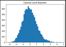
Let’s check this using python:

讓我們使用python檢查一下：

Steps:

腳步：

• Draw n samples from exponential distribution
  從指數分布中抽取n個樣本
• Normalize the sum of n samples
  歸一化n個樣本的總和
• Repeat above steps N times
  重復上述步驟N次
• Keep storing the normalized sum in sum_list
  繼續將歸一化的和存儲在sum_list中
• In the end, plot the histogram of the normalized sum_list
  最后，繪制歸一化的sum_list的直方圖
• The output closely follows Gaussian distribution, as shown below:
  輸出緊密遵循高斯分布，如下所示：

Similarly, there are several other distributions like Student t distribution, chi-squared distribution, F distribution etc which have strong dependence on the Gaussian distribution. For e.g. t-distribution is a result of infinite mixture of Gaussians leading to longer tails as compared to a Gaussian one.

同樣，還有其他一些分布，例如學生t分布，卡方分布，F分布等，它們對高斯分布有很強的依賴性。 例如，t分布是高斯混合的無限結果，與高斯相比，它導致更長的尾巴。

Properties of Gaussian Distribution:

高斯分布的性質：

1) Affine transformation:

1) 仿射變換：

It is a simple transformation of multiplying the random variable with a scalar ‘a’ and adding another scalar ‘b’ to it.

這是將隨機變量與標量“ a”相乘并向其添加另一個標量“ b”的簡單轉換。

The resulting distribution is Gaussian with mean:

結果分布為高斯，均值：

If X ~ N(𝜇, 𝜎2), then for any a,b ∈ ?,

如果X?N(𝜇，𝜎2)，那么對于任何a，b∈?，

a.X+b ~ N(a. 𝜇+b, a2.𝜎2)

a.X + b?N(a。𝜇 + b，a2.𝜎2)

Note that not all transformations result into Gaussian, for e.g. square of a Gaussian will not lead to Gaussian.

請注意，并非所有的變換都會產生高斯，例如，高斯的平方不會導致高斯。

2) Standardization:

2) 標準化：

If we have 2 sets of observations, each drawn from a normal distribution with different mean and sigma, then how do we compare the two observations to calculate the probabilities with respect to their population?

如果我們有兩組觀測值，每組觀測值均來自具有不同均值和sigma的正態分布，那么我們如何比較這兩個觀測值以計算其總體的概率？

Hence, we need to convert the observations mentioned above into Z score. This process is called as Standardization which adjusts the raw observation with respect to its mean and sigma of the population it is generated from and brings it onto a common scale

因此，我們需要將上述觀察值轉換為Z分數。 此過程稱為“標準化”，它根據原始觀測值的平均值和總和來調整原始觀測值，并將其放到一個通用范圍內

3) Conditional distribution: An important property of multivariate Gaussian is that if two sets of variables are jointly Gaussian, then the conditional distribution of one set conditioned on the other set is again Gaussian

3) 條件分布：多元高斯的一個重要屬性是，如果兩組變量聯合為高斯，則以另一組為條件的一組的條件分布又是高斯

4) Marginal distribution of the set is also a Gaussian

4)集合的邊際分布也是高斯分布

5) Gaussian distributions are self-conjugate i.e. given the Gaussian likelihood function, choosing the Gaussian prior will result in Gaussian posterior.

5)高斯分布是自共軛的，即給定高斯似然函數，選擇高斯先驗將導致高斯后驗。

6) Sum and difference of two independent Gaussian random variables is a Gaussian

6)兩個獨立的高斯隨機變量的和與差是一個高斯

Limitations of Gaussian Distributions:

高斯分布的局限性：

1. Simple Gaussian distribution fails to capture the below structure:
   簡單的高斯分布無法捕獲以下結構：

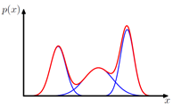
Such structure is better characterized by the linear combination of two Gaussians (also known as mixture of Gaussians). However, it's complex to estimate the parameters of such mixture of Gaussians.

通過兩個高斯線性組合(也稱為高斯混合)可以更好地描述這種結構。 但是，估計這種高斯混合參數很復雜。

2) Gaussian distribution is uni-modal, i.e. it fails to provide a good approximation to multi-modal distributions thereby restricting the range of distributions that it can represent adequately.

2)高斯分布是單峰分布，即它不能很好地近似多峰分布，從而限制了它可以充分表示的分布范圍。

3) Degrees of freedom grow quadratically with an increase in the number of dimensions. This results in high computational complexity in inverting such large covariance matrix.

3)自由度隨著尺寸數量的增加而平方增長。 在反轉這樣大的協方差矩陣時，這導致很高的計算復雜度。

Hope the post gives you a sneak peek into the world of Gaussian distributions.

希望這篇文章能使您對高斯分布的世界有所了解。

Happy Reading!!!

閱讀愉快！