XTS對象 (XTS Objects)

If you’re not using XTS objects to perform your forecasting in R, then you are likely missing out! The major benefits that we’ll explore throughout are that these objects are a lot easier to work with when it comes to modeling, forecasting, & visualization.

如果您沒有使用XTS對象在R中執行預測，那么您很可能會錯過！ 我們將始終探索的主要好處是，在建模，預測和可視化方面，這些對象更易于使用。

讓我們進入細節 (Let’s Get to The Details)

XTS objects are composed of two components. The first is a date index and the second of which is a traditional data matrix.

XTS對象由兩個組件組成。 第一個是日期索引，第二個是傳統數據矩陣。

Whether you want to predict churn, sales, demand, or whatever else, let’s get to it!

無論您是要預測客戶流失，銷售，需求還是其他，我們都可以開始吧！

The first thing you’ll need to do is create your date index. We do so using the seq function. Very simply this function takes what is your start date, the number of records you have or length, and then the time interval or by parameter. For us, the dataset starts with the following.

您需要做的第一件事是創建日期索引。 我們使用seq函數。 很簡單，此功能需要的只是你的開始日期，你有記錄的數目或長度，然后將時間間隔或by參數。 對于我們來說，數據集從以下開始。

days <- seq(as.Date("2014-01-01"), length = 668, by = "day")

Now that we have our index, we can use it to create our XTS object. For this, we will use the xts function.

現在我們有了索引，可以使用它來創建XTS對象。 為此，我們將使用xts函數。

Don’t forget to install.packages('xts') and then load the library! library(xts)

不要忘了先安裝install.packages('xts') ，然后加載庫！ library(xts)

Once we’ve done this we’ll make our xts call and pass along our data matrix, and then for the date index we will pass the index to the order.by option.

完成此操作后，我們將進行xts調用并傳遞數據矩陣，然后對于日期索引，我們會將索引傳遞給order.by選項。

sales_xts <- xts(sales, order.by = days)

讓我們與Arima建立預測 (Let’s Create a Forecast with Arima)

Arima stands for auto regressive integrated moving average. A very popular technique when it comes to time series forecasting. We could spend hours talking about ARIMA alone, but for this post, we’re going to give a high-level explanation and then jump directly into the application.

有馬代表自動回歸綜合移動平均線。 關于時間序列預測的一種非常流行的技術。 我們可能只花幾個小時來談論ARIMA，但是在這篇文章中，我們將給出一個高級的解釋，然后直接進入該應用程序。

AR：自回歸 (AR: Auto Regressive)

This is where we predict outcomes using lags or values from previous months. It may be that the outcomes of a given month have some dependency on previous values.

在這里，我們使用前幾個月的滯后或值來預測結果。 給定月份的結果可能與以前的值有一定的依賴性。

一：集成 (I: Integrated)

When it comes to time series forecasting, an implicit assumption is that our model depends on time in some capacity. This seems pretty obvious as we probably wouldn’t make our model time based otherwise ;). With that assumption out of the way, we need to understand where on the spectrum of dependence time falls in relation to our model. Yes, our model depends on time, but how much? Core to this is the idea of Stationarity; which means that the effect of time diminishes as time goes on.

在進行時間序列預測時，一個隱含的假設是我們的模型在某種程度上取決于時間。 這似乎很明顯，因為我們可能不會將模型時間設為其他時間；)。 有了這個假設，我們需要了解與我們的模型有關的依賴時間范圍。 是的，我們的模型取決于時間，但是多少？ 核心思想是平穩性 ； 這意味著隨著時間的流逝，時間的影響減弱。

Going deeper, the historical average of a dataset tends to be the best predictor of future outcomes… but there are certainly times when that’s not true.. can you think of any situations when the historical mean would not be the best predictor?

更深入地講，數據集的歷史平均值往往是未來結果的最佳預測因子……但是，在某些情況下，這是不正確的……您能想到歷史均值不是最佳預測因子的任何情況嗎？

• How about predicting sales for December? Seasonal Trends
  預測12月的銷售情況如何？ 季節性趨勢
• How about sales for a hyper-growth saas company? Consistent upward trends
  一家高速增長的saas公司的銷售情況如何？ 一致的上升趨勢

This is where the process of Differencing is introduced! Differencing is used to eliminate the effects of trends & seasonality.

這就是引入差分過程的地方！ 差異用于消除趨勢和季節性的影響。

MA：移動平均線 (MA: Moving Average)

the moving average model exists to deal with the error of your model.

存在移動平均模型以處理模型誤差。

讓我們開始建模吧！ (Let’s Get Modeling!)

火車/驗證拆分 (Train/Validation Split)

First things first, let’s break out our data into a training dataset and then what we’ll call our validation dataset.

首先，讓我們將數據分為訓練數據集，然后將其稱為驗證數據集。

What makes this different than other validation testing, like cross-validation testing is that here we break it out by time, breaking train up to a given point in time and breaking out validation for everything thereafter.

與其他驗證測試(例如交叉驗證測試)不同的是，這里我們按時間細分，將訓練分解到給定的時間點，然后對所有內容進行驗證。

train <- sales_xts[index(sales_xts) <= "2015-07-01"] 
validation <- sales_xts[index(sales_xts) > "2015-07-01"]

是時候建立模型了 (Time to Build a Model)

The auto.arima function incorporates the ideas we just spoke about to approximate the best arima model. I will detail the more hands-on approach in another post, but below I’ll explore the generation of an auto.arima model and how to use it to forecast.

auto.arima函數結合了我們剛才談到的想法，可以近似最佳arima模型。 我將在另一篇文章中詳細介紹更多的動手方法，但是下面我將探討auto.arima模型的生成以及如何使用它進行預測。

model <- auto.arima(train)

Now let’s generate a forecast. The same way we did before, we’ll create a date index and then create an xts object with the data matrix.

現在讓我們生成一個預測。 與之前相同，我們將創建一個日期索引，然后使用數據矩陣創建一個xts對象。

From here you will plot the validation data and then throw the forecast on top of the plot.

在這里，您將繪制驗證數據，然后將預測放在該圖的頂部。

forecast <- forecast(model, h = 121) 
forecast_dates <- seq(as.Date("2015-09-01"), length = 121, by = "day")forecast_xts <- xts(forecast$mean, order.by = forecast_dates)plot(validation, main = 'Forecast Comparison')lines(forecast_xts, col = "blue")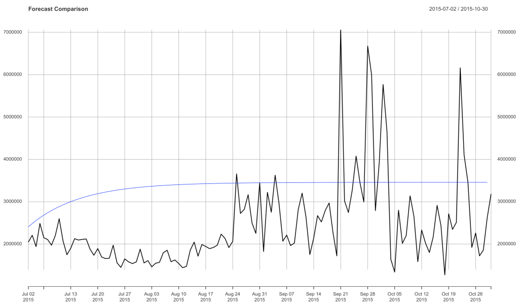

結論 (Conclusion)

I hope this was a helpful introduction to ARIMA forecasting. Be sure to let me know what’s helpful and any additional detail you’d like to learn about.

我希望這對ARIMA預測很有幫助。 請務必讓我知道有什么幫助以及您想了解的任何其他詳細信息。

If you found this helpful be sure to check out some of my other posts on datasciencelessons.com. Happy Data Science-ing!

如果您認為這有幫助，請務必在datasciencelessons.com上查看我的其他一些帖子。 快樂數據科學！