Save time, resources and stay healthy with data exploration that goes beyond means, distributions and correlations: Leverage PCA to see through the surface of variables. It saves time and resources, because it uncovers data issues before an hour-long model training and is good for a programmer’s health, since she trades off data worries with something more enjoyable. For example, a well-proven machine learning model might fail, because of one-dimensional data with insufficient variance or other related issues. PCA offers valuable insights that make you confident about data properties and its hidden dimensions.

超越均值，分布和相關性的數據探索可節省時間，資源并保持健康：利用PCA透視變量的表面。 它節省了時間和資源，因為它在一小時的模型訓練之前就發現了數據問題，并且對程序員的健康非常有益，因為她可以用更有趣的東西來權衡數據的煩惱。 例如，由于一維數據的方差不足或其他相關問題，一個經過充分驗證的機器學習模型可能會失敗。 PCA提供了寶貴的見解，使您對數據屬性及其隱藏維度充滿信心。

This article shows how to leverage PCA to understand key properties of a dataset, saving time and resources down the road which ultimately leads to a happier, more fulfilled coding life. I hope this post helps to apply PCA in a consistent way and understand its results.

本文展示了如何利用PCA來理解數據集的關鍵屬性，從而節省時間和資源，最終使編碼壽命更長壽，更令人滿意。 我希望這篇文章有助于以一致的方式應用PCA并了解其結果。

TL; DR (TL;DR)

PCA provides valuable insights that reach beyond descriptive statistics and help to discover underlying patterns. Two PCA metrics indicate 1. how many components capture the largest share of variance (explained variance), and 2., which features correlate with the most important components (factor loading). These metrics crosscheck previous steps in the project work flow, such as data collection which then can be adjusted. As a shortcut and ready-to-use tool, I provide the function do_pca() which conducts a PCA for a prepared dataset to inspect its results within seconds in this notebook or this script.

PCA提供了有價值的見解，這些見解超出了描述性統計數據的范圍，并有助于發現潛在的模式。 兩個PCA指標指示1.捕獲最大方差份額的成分( 解釋了方差 )，以及2.與最重要的成分相關的特征( 要素負載 )。 這些度量標準可以交叉檢查項目工作流程中的先前步驟 ，例如可以進行數據收集的調整。 作為一種快捷且易于使用的工具，我提供了do_pca()函數，該函數為準備好的數據集執行PCA，以在此筆記本或此腳本中在幾秒鐘內檢查其結果。

數據探索作為安全網 (Data exploration as a safety net)

When a project structure resembles the one below, the prepared dataset is under scrutiny in the 4. step by looking at descriptive statistics. Among the most common ones are means, distributions and correlations taken across all observations or subgroups.

當項目結構類似于以下結構時，通過查看描述性統計數據，將在第4步中仔細檢查準備的數據集。 最常見的是在所有觀察值或子組中采用的均值，分布和相關性。

Common project structure

共同的項目結構

1. Collection: gather, retrieve or load data
   收集：收集，檢索或加載數據
2. Processing: Format raw data, handle missing entries
   處理：格式化原始數據，處理缺失的條目
3. Engineering: Construct and select features
   工程：構造和選擇特征

4. Exploration: Inspect descriptives, properties

   探索：檢查描述，屬性

5. Modelling: Train, validate and test models
   建模：訓練，驗證和測試模型
6. Evaluation: Inspect results, compare models
   評估：檢查結果，比較模型

When the moment arrives of having a clean dataset after hours of work, makes many glances already towards the exciting step of applying models to the data. At this stage, around 80–90% of the project’s workload is done, if the data did not fell out of the sky, cleaned and processed. Of course, the urge is strong for modeling, but here are two reasons why a thorough data exploration saves time down the road:

在經過數小時的工作后，有了一個干凈的數據集的時刻到來時，已經將許多目光投向了將模型應用于數據的令人興奮的步驟。 在這個階段，如果數據沒有從天而降，清理和處理，則大約完成了項目工作量的80–90％。 當然，建模的沖動很強烈，但是這里有 徹底的數據探索可以節省時間的兩個原因：

1. catch coding errors → revise feature engineering (step 3)

   捕獲編碼錯誤 →修改特征工程(步驟3)

2. identify underlying properties → rethink data collection (step 1), preprocessing (step 2) or feature engineering (step 3)

   識別基礎屬性 →重新考慮數據收集(步驟1)，預處理(步驟2)或特征工程(步驟3)

Wondering about underperforming models due to underlying data issues after a few hours into training, validating and testing is like a photographer on the set, not knowing how their models might look like. Therefore, the key message is to see data exploration as an opportunity to get to know your data, understanding its strength and weaknesses.

經過數小時的培訓，驗證和測試后，由于底層數據問題而導致模型表現不佳的問題，就像布景中的攝影師一樣，不知道其模型會是什么樣子。 因此，關鍵信息是將數據探索視為了解您的數據 ，了解其優勢和劣勢的機會。

Descriptive statistics often reveal coding errors. However, detecting underlying issues likely requires more than that. Decomposition methods such as PCA help to identify these and enable to revise previous steps. This ensures a smooth transition to model building.

描述性統計通常會揭示編碼錯誤。 但是，要發現潛在的問題可能還需要更多。 分解方法(例如PCA)有助于識別這些方法，并可以修改以前的步驟。 這樣可以確保順利過渡到模型構建。

用PCA看表面之下 (Look beneath the surface with PCA)

Large datasets often require PCA to reduce dimensionality anyway. The method as such captures the maximum possible variance across features and projects observations onto mutually uncorrelated vectors, called components. Still, PCA serves other purposes than dimensionality reduction. It also helps to discover underlying patterns across features.

無論如何，大型數據集通常需要PCA來減少維數。 這樣的方法捕獲了整個特征的最大可能方差，并將觀測值投影到互不相關的向量(稱為分量)上。 盡管如此，PCA還可以實現降維以外的其他目的。 它還有助于發現跨功能的基礎模式。

To focus on the implementation in Python instead of methodology, I will skip describing PCA in its workings. There exist many great resources about it that I refer to those instead:

為了專注于Python的實現而不是方法論，我將不介紹PCA的工作原理。 我有很多關于它的大量資源可供參考：

• Animations showing PCA in action: https://setosa.io/ev/principal-component-analysis/

  演示PCA動作的動畫： https ： //setosa.io/ev/principal-component-analysis/

• PCA explained in a family conversation: https://stats.stackexchange.com/a/140579

  PCA在一次家庭對話中進行了解釋： https ： //stats.stackexchange.com/a/140579

• Smith [2]. A tutorial on principal components analysis: Accessible here.

  史密斯[2]。 主成分分析教程： 可在此處訪問 。

Two metrics are crucial to make sense of PCA for data exploration:

要使PCA對數據??探索有意義，有兩個指標至關重要：

1. Explained variance measures how much a model can reflect the variance of the whole data. Principle components try to capture as much of the variance as possible and this measure shows to what extent they can do that. It helps to see Components are sorted by explained variance, with the first one scoring highest and with a total sum of up to 1 across all components.

1.解釋方差 度量模型可以反映多少整體數據方差。 主成分嘗試捕獲盡可能多的方差，此度量表明它們可以做到的程度。 有助于按解釋的方差對組件進行排序，第一個得分最高，所有組件的總和最高為1。

2. Factor loading indicates how much a variable correlates with a component. Each component is made of a linear combination of variables, where some might have more weight than others. Factor loadings indicate this as correlation coefficients, ranging from -1 to 1, and make components interpretable.

2.因子加載 指示變量與組件的相關程度。 每個組件均由變量的線性組合組成，其中某些組件可能比其他組件具有更大的權重。 因子加載將此表示為相關系數，范圍為-1至1，并使組件可解釋。

The upcoming sections apply PCA to exciting data from a behavioral field experiment and guide through using these metrics to enhance data exploration.

接下來的部分將PCA應用于來自行為現場實驗的令人興奮的數據，并指導如何使用這些指標來增強數據探索。

負荷數據：砂礫的隨機教育干預(Alan等，2019) (Load data: A Randomized Educational Intervention on Grit (Alan et al., 2019))

The iris dataset served well as a canonical example of several PCA. In an effort to be diverse and using novel data from a field study, I rely on replication data from Alan et al. [1]. I hope this is appreciated. It comprises data from behavioral experiments at Turkish schools, where 10 year olds took part in a curriculum to improve a non-cognitive skill called grit which defines as perseverance to pursue a task. The authors sampled individual characteristics and conducted behavioral experiments to measure a potential treatment effect between those receiving the program ( grit == 1) and those taking part in a control treatment ( grit == 0).

虹膜數據集很好地代表了幾個PCA。 為了實現多樣性并使用來自實地研究的新穎數據，我依靠Alan等人的復制數據。 [1]。 希望我對此表示贊賞。 它包含來自土耳其學校的行為實驗的數據，土耳其學校的10歲兒童參加了一項課程，以提高名為grit的非認知技能，該技能定義為堅持執業的毅力。 作者對個人特征進行了采樣，并進行了行為實驗，以測量接受該程序的人( grit == 1 )與參與對照治療的人( grit == 0 )之間的潛在治療效果。

The following loads the data from an URL and stores it as a pandas dataframe.

以下內容從URL加載數據并將其存儲為pandas數據框。

# To load data from Harvard Dataverse
import io 
import requests# load exciting data from URL (at least something else than Iris)
url = ‘https://dataverse.harvard.edu/api/access/datafile/3352340?gbrecs=false'
s = requests.get(url).content# store as dataframe
df_raw = pd.read_csv(io.StringIO(s.decode(‘utf-8’)), sep=’\t’)

預處理和特征工程 (Preprocessing and feature engineering)

For PCA to work, the data needs to be numeric, without missings, and standardized. I put all steps into one function ( clean_data) which returns a dataframe with standardized features. and conduct steps 1 to 3 of the project work flow (collecting, processing and engineering). To begin with, import necessary modules and packages.

為了使PCA能夠正常工作，數據必須是數字化的，無遺漏的并且是標準化的。 我將所有步驟都放在一個函數( clean_data )中，該函數返回具有標準化功能的數據框。 并執行項目工作流程的第1步到第3步(收集，處理和工程)。 首先，導入必要的模塊和軟件包。

import pandas as pd
import numpy as np# sklearn module
from sklearn.decomposition import PCA# plots
import matplotlib.pyplot as plt
import seaborn as sns
# seaborn settings
sns.set_style("whitegrid")
sns.set_context("talk")# imports for function
from sklearn.preprocessing import StandardScaler
from sklearn.impute import SimpleImputer

Next, the clean_data() function is defined. It gives a shortcut to transform the raw data into a prepared dataset with (i.) selected features, (ii.) missings replaced by column means, and (iii.) standardized variables.

接下來，定義clean_data()函數。 它提供了一種將原始數據轉換為準備好的數據集的捷徑，該數據集具有(i。)選定要素，(ii。)缺失值被列均值替換，以及(iii。)標準化變量。

Note about selected features: I selected features in (iv.) according to their replication scripts, accessible on Harvard Dataverse and solely used sample 2 (“sample B” in the publicly accessible working paper). To be concise, refer to the paper for relevant descriptives (p. 30, Table 2).

有關所選功能的說明：我在(iv。)中根據其復制腳本選擇了功能，這些功能可在Harvard Dataverse和單獨使用的示例2(可公開訪問的工作文件中的“示例B”)中進行訪問。 為簡明起見，請參閱本文中的相關說明(表2，第30頁)。

Preparing the data takes one line of code (v).

準備數據需要一行代碼(v)。

def clean_data(data, select_X=None, impute=False, std=False): 
    """Returns dataframe with selected, imputed 
       and standardized features
    
    Input
          data: dataframe
          select_X: list of feature names to be selected (string)
          impute: If True impute np.nan with mean
          std: If True standardize data
          
    Return
        dataframe: data with selected, imputed 
                   and standardized features    
    """
    
    # (i.) select features
    if select_X is not None:
        data = data.filter(select_X, axis='columns')
        print("\t>>> Selected features: {}".format(select_X))
    else:
        # store column names
        select_X = list(data.columns)
    
    # (ii.) impute with mean 
    if impute:
        imp = SimpleImputer()
        data = imp.fit_transform(data)
        print("\t>>> Imputed missings")
    
    # (iii.) standardize 
    if std:
        std_scaler = StandardScaler()
        data = std_scaler.fit_transform(data)
        print("\t>>> Standardized data")
    
    return pd.DataFrame(data, columns=select_X)#  (iv.) select relevant features in line with Alan et al. (2019)
selected_features = ['grit', 'male', 'task_ability', 'raven', 'grit_survey1', 'belief_survey1', 'mathscore1', 'verbalscore1', 'risk', 'inconsistent']# (v.) select features, impute missings and standardize
X_std = clean_data(df_raw, selected_features, impute=True, std=True)

Now, the data is ready for exploration.

現在，數據已準備好進行探索。

碎石圖和因子加載：解釋PCA結果 (Scree plots and factor loadings: Interpret PCA results)

A PCA yields two metrics that are relevant for data exploration: Firstly, how much variance each component explains (scree plot), and secondly how much a variable correlates with a component (factor loading). The following sections provide a practical example and guide through the PCA output with a scree plot for explained variance and a heatmap on factor loadings.

PCA產生兩個與數據探查相關的指標：首先，每個組件可以解釋多少差異(scree圖)，其次，變量與某個組件有多少關聯(因子加載)。 以下各節提供了一個實際示例，并通過一個scree圖表指導了PCA輸出，以提供解釋的方差和因子負載的熱圖。

解釋方差顯示跨變量的維數 (Explained variance shows the number of dimensions across variables)

Nowadays, data is abundant and the size of datasets continues to grow. Data scientists routinely deal with hundreds of variables. However, are these variables worth their memory? Put differently: Does a variable capture unique patterns or does it measure similar properties already reflected by other variables?

如今，數據非常豐富，數據集的規模也在不斷增長。 數據科學家通常處理數百個變量。 但是，這些變量值得記憶嗎？ 換句話說：變量是捕獲唯一模式還是測量其他變量已經反映的相似屬性？

PCA might answer this through the metric of explained variance per component. It details the number of underlying dimensions on which most of the variance is observed.

PCA可以通過解釋每個組件的差異度量來回答這一問題。 它詳細說明了可觀察到大部分差異的基礎維數。

The code below initializes a PCA object from sklearn and transforms the original data along the calculated components (i.). Thereafter, information on explained variance is retrieved (ii.) and printed (iii.).

下面的代碼從sklearn初始化PCA對象，并沿計算的分量(i。)轉換原始數據。 此后，檢索(ii。)有關解釋的方差的信息并進行打印(iii。)。

# (i.) initialize and compute pca
pca = PCA()
X_pca = pca.fit_transform(X_std)# (ii.) get basic info
n_components = len(pca.explained_variance_ratio_)
explained_variance = pca.explained_variance_ratio_
cum_explained_variance = np.cumsum(explained_variance)
idx = np.arange(n_components)+1df_explained_variance = pd.DataFrame([explained_variance, cum_explained_variance], 
                                     index=['explained variance', 'cumulative'], 
                                     columns=idx).Tmean_explained_variance = df_explained_variance.iloc[:,0].mean() # calculate mean explained variance# (iii.) Print explained variance as plain text
print('PCA Overview')
print('='*40)
print("Total: {} components".format(n_components))
print('-'*40)
print('Mean explained variance:', round(mean_explained_variance,3))
print('-'*40)
print(df_explained_variance.head(20))
print('-'*40)PCA Overview 
======================================== 
Total: 10 components 
---------------------------------------- 
Mean explained variance: 0.1 
---------------------------------------- 
explained variance cumulative 
1 0.265261 0.265261 
2 0.122700 0.387962 
3 0.113990 0.501951 
4 0.099139 0.601090 
5 0.094357 0.695447 
6 0.083412 0.778859 
7 0.063117 0.841976 
8 0.056386 0.898362 
9 0.052588 0.950950 
10 0.049050 1.000000 
----------------------------------------

Interpretation: The first component makes up for around 27% of the explained variance. This is relatively low as compared to other datasets, but no matter of concern. It simply indicates that a major share (100%–27%=73%) of observations distributes across more than one dimension. Another way to approach the output is to ask: How much components are required to cover more than X% of the variance? For example, I want to reduce the data’s dimensionality and retain at least 90% variance of the original data. Then I would have to include 9 components to reach at least 90% and even have 95% of explained variance covered in this case. With an overall of 10 variables in the original dataset, the scope to reduce dimensionality is limited. Additionally, this shows that each of the 10 original variables adds somewhat unique patterns and limitedly repeats information from other variables.

解釋：第一部分占解釋差異的約27％。 與其他數據集相比，這相對較低，但無需擔心。 它只是表明觀察的主要部分(100％–27％= 73％)分布在多個維度上。 處理輸出的另一種方法是問：要覆蓋超過X％的方差需要多少分量？ 例如，我想減少數據的維數并保留原始數據的至少90％的差異。 然后，在這種情況下，我將必須包含9個組成部分才能至少達到90％，甚至還要涵蓋95％的解釋方差。 在原始數據集中總共有10個變量，減少維數的范圍是有限的。 此外，這表明10個原始變量中的每個變量都添加了一些獨特的模式，并有限地重復了來自其他變量的信息。

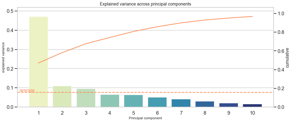
To give another example, I list explained variance of “the” wine dataset:

再舉一個例子，我列出了“ the” 葡萄酒數據集的解釋方差：

PCA Overview: Wine dataset 
======================================== 
Total: 13 components 
---------------------------------------- 
Mean explained variance: 0.077 
---------------------------------------- 
explained variance cumulative 
1 0.361988 0.361988 
2 0.192075 0.554063 
3 0.111236 0.665300 
4 0.070690 0.735990 
5 0.065633 0.801623 
6 0.049358 0.850981 
7 0.042387 0.893368 
8 0.026807 0.920175 
9 0.022222 0.942397 
10 0.019300 0.961697 
11 0.017368 0.979066 
12 0.012982 0.992048 
13 0.007952 1.000000 
----------------------------------------

Here, 8 out of 13 components suffice to capture at least 90% of the original variance. Thus, there is more scope to reduce dimensionality. Furthermore, it indicates that some variables do not contribute much to variance in the data.

在這里，13個成分中的8個足以捕獲至少90％的原始方差。 因此，存在減小尺寸的更大范圍。 此外，它表明某些變量對數據方差的貢獻不大。

Instead of plain text, a scree plot visualizes explained variance across components and informs about individual and cumulative explained variance for each component. The next code chunk creates such a scree plot and includes an option to focus on the first X components to be manageable when dealing with hundreds of components for larger datasets (limit).

代替純文本， 碎石圖可直觀顯示各個組件之間的已解釋方差，并告知每個組件的單個和累積已解釋方差。 下一個代碼塊創建了這樣的scree圖，并包括一個選項，該選項著重于在處理較大數據集的數百個組件( limit )時可管理的前X個組件。

#limit plot to x PC
limit = int(input("Limit scree plot to nth component (0 for all) > "))
if limit > 0:
    limit_df = limit
else:
    limit_df = n_componentsdf_explained_variance_limited = df_explained_variance.iloc[:limit_df,:]#make scree plot
fig, ax1 = plt.subplots(figsize=(15,6))ax1.set_title('Explained variance across principal components', fontsize=14)
ax1.set_xlabel('Principal component', fontsize=12)
ax1.set_ylabel('Explained variance', fontsize=12)ax2 = sns.barplot(x=idx[:limit_df], y='explained variance', data=df_explained_variance_limited, palette='summer')
ax2 = ax1.twinx()
ax2.grid(False)ax2.set_ylabel('Cumulative', fontsize=14)
ax2 = sns.lineplot(x=idx[:limit_df]-1, y='cumulative', data=df_explained_variance_limited, color='#fc8d59')ax1.axhline(mean_explained_variance, ls='--', color='#fc8d59') #plot mean
ax1.text(-.8, mean_explained_variance+(mean_explained_variance*.05), "average", color='#fc8d59', fontsize=14) #label y axismax_y1 = max(df_explained_variance_limited.iloc[:,0])
max_y2 = max(df_explained_variance_limited.iloc[:,1])
ax1.set(ylim=(0, max_y1+max_y1*.1))
ax2.set(ylim=(0, max_y2+max_y2*.1))plt.show()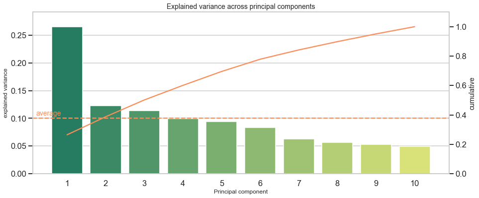

A scree plot might show distinct jumps from one component to another. For example, when the first component captures disproportionately more variance than others, it could be a sign that variables inform about the same underlying factor or do not add additional dimensions, but say the same thing from a marginally different angle.

碎石圖可能顯示從一個組件到另一個組件的明顯跳躍。 例如，當第一個組件比其他組件更多地捕獲方差時，這可能表明變量告知了相同的潛在因素或未添加其他維度，而是從稍微不同的角度說了同樣的話。

To give a direct example and to get a feeling for how distinct jumps might look like, I provide the scree plot of the Boston house prices dataset:

為了給出一個直接的例子并了解不同的跳躍可能是什么樣子，我提供了波士頓房價數據集的稀疏圖：

PCA節省時間的兩個原因 (Two Reasons why PCA saves time down the road)

Assume you have hundreds of variables, apply PCA and discover that over much of the explained variance is captured by the first few components. This might hint at a much lower number of underlying dimensions than the number of variables. Most likely, dropping some hundred variables leads to performance gains for training, validation and testing. There will be more time left to select a suitable model and refine it than to wait for the model itself to discover lack of variance behind several variables.

假設您有數百個變量，應用PCA并發現前幾個組件捕獲了大部分解釋的方差。 這可能暗示底層維數要比變量數少得多 。 最有可能的是，減少數百個變量可以提高培訓，驗證和測試的性能。 與等待模型本身發現幾個變量背后的方差相比，剩下更多的時間來選擇合適的模型并進行優化。

In addition to this, imagine that the data was constructed by oneself, e.g. through web scraping, and the scraper extracted pre-specified information from a web page. In that case, the retrieved information could be one-dimensional, when the developer of the scraper had only few relevant items in mind, but forgot to include items that shed light on further aspects of the problem setting. At this stage, it might be worthwhile to go back to the first step of the work flow and adjust data collection.

除此之外，假設數據是由自己構建的，例如通過Web抓取，并且該抓取器從網頁中提取了預先指定的信息。 在那種情況下，當刮板的開發人員只考慮很少的相關項目時， 檢索到的信息可能是一維的 ，但是卻忘了包含那些可以闡明問題更多方面的信息。 在此階段，可能值得回到工作流程的第一步并調整數據收集 。

通過功能和組件之間的關聯發現潛在因素 (Discover underlying factors with correlations between features and components)

PCA offers another valuable statistic besides explained variance: The correlation between each principle component and a variable, also called factor loading. This statistic facilitates to grasp the dimension that lies behind a component. For example, a dataset includes information about individuals such as math score, reaction time and retention span. The overarching dimension would be cognitive skills and a component that strongly correlates with these variables can be interpreted as the cognitive skill dimension. Similarly, another dimension could be non-cognitive skills and personality, when the data has features such as self-confidence, patience or conscientiousness. A component that captures this area highly correlates with those features.

除了解釋的方差外，PCA還提供了另一個有價值的統計數據：每個主成分與變量之間的相關性，也稱為因子加載。 此統計信息有助于掌握組件后面的尺寸。 例如，數據集包括有關個人的信息，例如數學分數，React時間和保留期。 最重要的方面是認知技能，與這些變量密切相關的組件可以解釋為認知技能。 同樣，當數據具有自信心，耐心或盡責性等特征時，另一個維度可能是非認知技能和個性。 捕獲該區域的組件與這些功能高度相關。

The following code creates a heatmap to inspect these correlations, also called factor loading matrix.

以下代碼創建了一個熱圖來檢查這些相關性，也稱為因子加載矩陣。

# adjust y-axis size dynamically
size_yaxis = round(X_std.shape[1] * 0.5)
fig, ax = plt.subplots(figsize=(8,size_yaxis))# plot the first top_pc components
top_pc = 3
sns.heatmap(df_c.iloc[:,:top_pc], annot=True, cmap="YlGnBu", ax=ax)
plt.show()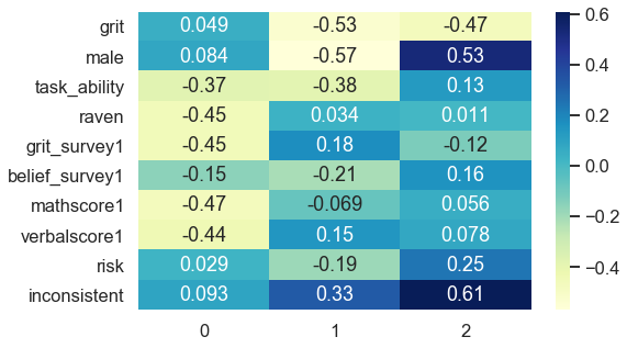

The first component strongly negatively associates with task ability, reasoning score (raven), math score, verbal score and positively links to beliefs about being gritty (grit_survey1). Summarizing this into a common underlying factor is subjective and requires domain knowledge. In my opinion, the first component mainly captures cognitive skills.

第一個組件與任務能力，推理分數( raven )，數學分數，語言分數強烈負相關，并與堅韌不拔的信念( grit_survey1 )呈正相關。 將其概括為常見的基本因素是主觀的，并且需要領域知識。 我認為，第一個組成部分主要是捕獲認知技能。

The second component correlates negatively with receiving the treatment (grit), gender (male) and positively relates to being inconsistent. Interpreting this dimension is less clear-cut and much more challenging. Nevertheless, it accounts for 12% of explained variance instead of 27% like the first component, which results in less interpretable dimensions as it spans slightly across several topical areas. All components that follow might be analogously difficult to interpret.

第二部分與接受治療( 沙粒 )負相關，與性別( 男性 )負相關，與前后矛盾呈正相關。 解釋這個維度不太明確，更具挑戰性。 但是，它占解釋差異的12％，而不是像第一個組成部分那樣占27％，這導致解釋性較小，因為它跨幾個主題區域。 類似地，后續的所有組件也可能難以解釋。

Evidence that variables capture similar dimensions could be uniformly distributed factor loadings. One example which inspired this article is on of my projects where I relied on Google Trends data and self-constructed keywords about a firm’s sustainability. A list of the 15th highest factor loadings for the first principle component revealed loadings ranging from 0.12 as the highest value to 0.11 as the lowest loading of all 15. Such a uniform distribution of factor loadings could be an issue. This especially applies when data is self-collected and someone preselected what is being considered for collection. Adjusting this selection might add dimensionality to your data which possibly improves model performance at the end.

變量捕獲相似維度的證據可能是均勻分布的因子載荷。 啟發本文的一個例子是在我的項目中 ，我依靠Google趨勢數據和關于公司可持續性的自建關鍵字。 第一個主成分的第15個最高因子載荷列表顯示，載荷從最大值15中的0.12到所有15中最低載荷中的0.11不等。這樣的因子載荷的均勻分布可能是一個問題。 當數據是自我收集并且有人預先選擇要收集的數據時，這尤其適用。 調整此選擇可能會增加數據的維度，從而可能最終改善模型性能。

PCA節省時間的另一個原因 (Another reason why PCA saves time down the road)

If the data was self-constructed, the factor loadings show how each feature contributes to an underlying dimension, which helps to come up with additional perspectives on data collection and what features or dimensions could add valuable variance. Rather than blind guessing which features to add, factor loadings lead to informed decisions for data collection. They may even be an inspiration in the search for more advanced features.

如果數據是自構造的，則因子加載將顯示每個要素如何對基礎維度做出貢獻，這有助于提出 關于數據收集的其他觀點 以及哪些要素或維度可以增加有價值的差異。 而不是盲目猜測要添加哪些功能，因子加載可以導致 明智的數據收集決策 。 它們甚至可能是尋求更高級功能的靈感。

結論 (Conclusion)

All in all, PCA is a flexible instrument in the toolbox for data exploration. Its main purpose is to reduce complexity of large datasets. But it also serves well to look beneath the surface of variables, discover latent dimensions and relate variables to these dimensions, making them interpretable. Key metrics to consider are explained variance and factor loading.

總而言之，PCA是工具箱中用于數據探索的靈活工具。 其主要目的是降低大型數據集的復雜性。 但是，它也可以很好地用于查看變量的表面，發現潛在維度并將變量與這些維度相關聯，從而使它們易于解釋。 要考慮的關鍵指標是方差和因子加載 。

This article shows how to leverage these metrics for data exploration that goes beyond averages, distributions and correlations and build an understanding of underlying properties of the data. Identifying patterns across variables is valuable to rethink previous steps in the project workflow, such as data collection, processing or feature engineering.

本文展示了如何利用這些指標進行超出平均值，分布和相關性的數據探索，并加深對數據基本屬性的理解。 跨變量識別模式對于重新思考項目工作流中的先前步驟(例如數據收集，處理或功能設計)非常重要。

Thanks for reading! I hope you find it as useful as I had fun to write this guide. I am curious of your thoughts on this matter. If you have any feedback I highly appreciate your feedback and look forward receiving your message.

謝謝閱讀！ 希望您覺得它和我編寫本指南一樣有用。 我很好奇你對此事的想法。 如果您有任何反饋意見，我將非常感謝您的反饋意見，并期待收到您的消息 。

附錄 (Appendix)

訪問Jupyter筆記本 (Access the Jupyter Notebook)

I applied PCA to even more exemplary datasets like Boston housing market, wine and iris using do_pca(). It illustrates how PCA output looks like for small datasets. Feel free to download my notebook or script.

我使用do_pca()將PCA應用于更多示例性數據集，例如波士頓住房市場，葡萄酒和鳶尾花。 它說明了小型數據集的PCA輸出外觀。 隨時下載我的筆記本或腳本 。

有關因子分析與PCA的注意事項 (Note on factor analysis vs. PCA)

A rule of thumb formulated here states: Use PCA if you want to reduce your correlated observed variables to a smaller set of uncorrelated variables and use factor analysis to test a model of latent factors on observed variables.

這里規定的經驗法則是：如果要將相關的觀察變量減少為較小的一組不相關變量，請使用PCA，并使用因子分析來測試觀察變量上的潛在因子模型。

Even though this distinction is scientifically correct, it becomes less relevant in an applied context. PCA relates closely to factor analysis which often leads to similar conclusions about data properties which is what we care about. Therefore, the distinction can be relaxed for data exploration. This post gives an example in an applied context and another example with hands-on code for factor analysis is attached in the notebook.

即使這種區別在科學上是正確的，但在實際應用中它的重要性就降低了。 PCA與因子分析密切相關，因子分析通常會得出我們關心的關于數據屬性的相似結論。 因此，可以放寬對數據探索的區分。 這篇文章給出了一個應用上下文中的示例， 筆記本中還附有另一個具有動因分析代碼的示例。

Finally, for those interested in the differences between factor analysis and PCA refer to this post. Note, that throughout this article I never used the term latent factor to be precise.

最后，對于那些對因子分析和PCA之間的差異感興趣的人，請參考這篇文章 。 請注意，在本文中，我從未使用術語“ 潛在因子”來精確。