背景 (Background)

Retailers typically have a wealth of customer transaction data which consists of the type of items purchased by a customer, their value and the date they were purchased. Unless the retailer has a loyalty rewards system, they may not have demographic information on their customers such as height, age, gender and address. Thus, in order to make suggestions on what this customer might want to buy in the future, i.e which products to recommend to a customer, this has to be based on their purchase history and information on the purchase history of other customers.

零售商通常擁有大量的客戶交易數據，這些數據包括客戶購買的商品的類型，其價值和購買日期。 除非零售商具有忠誠度獎勵制度，否則他們可能沒有客戶的人口統計信息，例如身高，年齡，性別和地址。 因此，為了提出關于該顧客將來可能想要購買什么的建議，即向顧客推薦哪些產品，這必須基于他們的購買歷史和關于其他顧客的購買歷史的信息。

In collaborative filtering, recommendations are made to customers based on finding similarities between the purchase history of customers. So, if Customers A and B both purchase Product A, but customer B also purchases Product B, then it is likely that customer A may also be interested in Product B. This is a very simple example and there are various algorithms that can be used to find out how similar customers are in order to make recommendations.

在協同過濾中 ，會根據發現客戶購買歷史之間的相似性來向客戶提出建議。 因此，如果客戶A和客戶B都購買了產品A，但客戶B也購買了產品B，則客戶A可能也對產品B感興趣。這是一個非常簡單的示例，可以使用多種算法找出相似的客戶以提出建議。

One such algorithm is k-nearest neighbour where the objective is to find k customers that are most similar to the target customer. It involves choosing a k and a similarity metric (with Euclidean distance being most common). The basis of this algorithm is that points that are closest in space to each other are also likely to be most similar to each other.

一種這樣的算法是k最近鄰居 ，其目的是找到與目標客戶最相似的k客戶。 它涉及選擇k和相似性度量(以歐幾里得距離最為常見)。 該算法的基礎是，在空間上彼此最接近的點也可能彼此最相似。

Another techinque is to use basket analysis or association rules. In this method, the aim is to find out which items are bought together (put in the same basket) and the frequency of this purchase. The output of this algorithm is a series of if-then rules i.e. if a customer buys a candle, then they are also likely to buy matches. Association rules can assist retailers with the following:

另一種技術是使用購物籃分析或關聯規則。 在這種方法中，目的是找出一起購買的物品(放在同一籃子中)和購買的頻率。 該算法的輸出是一系列的if-then規則，即，如果客戶購買了一支蠟燭，那么他們也很可能會購買火柴。 關聯規則可以協助零售商進行以下工作：

• Modifying store layout where associated items are stocked together;
  修改將相關物料存放在一起的商店布局；
• Sending emails to customers with recommendations on products to purchase based on their previous purchase (i.e. we noticed you bought a candle, perhaps these matches may interest you?); and
  向客戶發送電子郵件，并根據他們先前的購買建議購買產品(即，我們注意到您購買了一支蠟燭，也許這些匹配可能會讓您感興趣？)； 和
• Insights into customer behaviour
  洞察客戶行為

Let’s now apply association rules to a dummy dataset

現在讓我們將關聯規則應用于虛擬數據集

數據集 (The dataset)

A dataset of 2,178,282 observations/rows and 16 variables/features was provided.

提供了2,178,282個觀測/行和16個變量/特征的數據集。

The first thing I did with this dataset was quickly check for any missing values or NAs as per follows. As shown below, no missing values were found.

我對此數據集所做的第一件事是按照以下步驟快速檢查是否有任何缺失值或NA。 如下所示，未找到缺失值。

Now the variables were all either read in as numeric or string variables. In order to meaningfully interpret categorical variables, they need to be changed to factors. As such, the following changes were made.

現在，所有變量都以數字或字符串變量形式讀入。 為了有意義地解釋分類變量，需要將其更改為因子。 因此，進行了以下更改。

retail <- retail %>% 
  mutate(MerchCategoryName = as.factor(MerchCategoryName)) %>%
  mutate(CategoryName = as.factor(CategoryName)) %>% 
  mutate(SubCategoryName = as.factor(SubCategoryName)) %>%
  mutate(StoreState = as.factor(StoreState)) %>%
  mutate(OrderType = as.factor(OrderType)) %>% 
  mutate (BasketID = as.numeric(BasketID)) %>% 
  mutate(MerchCategoryCode = as.numeric(MerchCategoryCode)) %>%
  mutate(CategoryCode = as.numeric(CategoryCode)) %>% 
  mutate(SubCategoryCode = as.numeric(SubCategoryCode)) %>% 
  mutate(ProductName = as.factor(ProductName))

Then, all the numeric variables were summarised into their five-point summary (min, median, max, std dev., and mean) to identify any outliers within the data. By running this summary, it was found that the features MerchCategoryCode, CategoryCode, and SubCategoryCode contained a large number of NAs. Upon further inspection, it was found that the majority of these code values contained digits; however, the ones that had been converted to NAs contained characters such as “Freight” or the letter “C”. As these codes are not related to customer purchases, these observations were removed.

然后，將所有數值變量匯總到其五點匯總中(最小值，中位數，最大值，標準偏差和均值)，以識別數據中的任何異常值。 通過運行這個總結，發現特征MerchCategoryCode，CategoryCode和 SubCategoryCode包含了大量的NAS。 經過進一步檢查，發現這些代碼值中的大多數包含數字。 但是，已轉換為NA的字母包含“運費”或字母“ C”之類的字符。 由于這些代碼與客戶購買無關，因此刪除了這些觀察結果。

Negative gross sales and negative quantity indicate either erroneous values or customer returns. This may be interesting information; however, it is not related to our objective of analysis and as such these observations were omitted.

負銷售總額和負數量表示錯誤的價值或客戶退貨。 這可能是有趣的信息。 但是，這與我們的分析目標無關，因此省略了這些觀察。

數據探索 (Data Exploration)

It is always a good idea to explore the data to see if you can see any trends or patterns within the dataset. Later on, you can use an algorithm/machine learning model to validate these trends.

探索數據以查看是否可以看到數據集中的任何趨勢或模式始終是一個好主意。 稍后，您可以使用算法/機器學習模型來驗證這些趨勢。

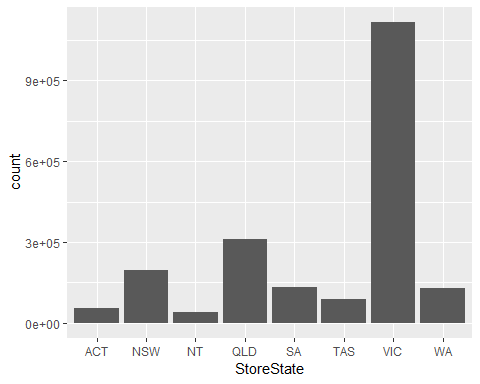
The graph below shows me that the highest number of transactions come from Victoria followed by Queensland. If a retailer wants to know where to increase sales then this plot may be useful as the number of sales are proportionately low in all other states.

下圖顯示了交易量最高的國家是維多利亞州，其次是昆士蘭州。 如果零售商想知道在哪里增加銷售額，那么該圖可能很有用，因為在所有其他州，銷售額均成比例降低。

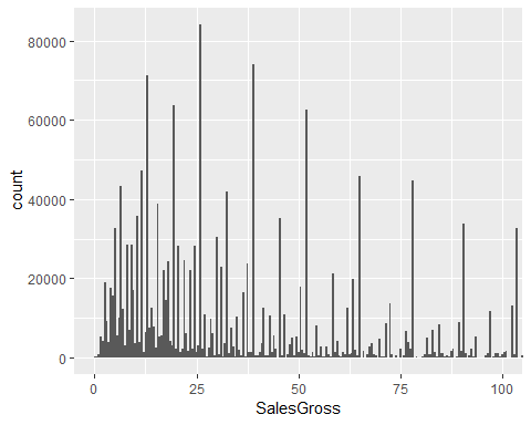
The below plot shows us that most gross sales values around >0-$40 (median is $37.60).

下圖顯示了大多數銷售總額> 0- $ 40(中位數為$ 37.60)。

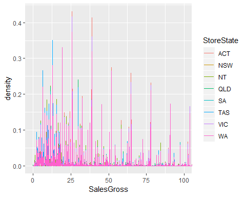
We can also see this plot by state as below. However, the transactions from Victoria and Queensland seem to cover up information for other states. Boxplots may be better for visualisation.

我們還可以按狀態查看此圖，如下所示。 但是，維多利亞州和昆士蘭州的交易似乎掩蓋了其他州的信息。 箱線圖可能更適合可視化。

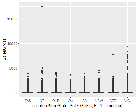
The below boxplots (though hard to see due to the scale being extended by the outliers) show that most sales across all states are close to the overall median. There in an abnormally high outlier for NT and a couple for VIC. For our purpose, since we are only interested in understanding which products do customers buy together in order to make recommendations, we do not need to deal with these outliers.

下面的方框圖(由于異常值擴大了規模，因此很難看到)表明，所有州的大多數銷售額都接近整體中位數。 NT異常高，VIC異常高。 就我們的目的而言，由于我們只想了解客戶一起購買哪些產品以提出建議，因此我們不需要處理這些異常值。

Now that we have had a look at sales by state. Let’s try and get a better understanding of the products purchased by customers.

現在，我們已經按州查看了銷售額。 讓我們嘗試更好地了解客戶購買的產品。

The plot below is coloured based on the frequency of purchases per item. Lighter shades of blue indicate higher frequencies.

下圖是根據每件物品的購買頻率著色的。 較淺的藍色陰影表示頻率較高。

Some key takeaways are:

一些關鍵要點是：

• No sales for team sports in ACT, NSW, SA, and WA — could be due to these products not being stocked there or perhaps they need to be marketed better
  ACT，NSW，SA和WA的團隊運動沒有銷售-可能是因為這些產品沒有在那里庫存，或者可能需要更好地銷售
• No sales for ski products in ACT, NSW, SA, and WA. I find this quite shocking as NSW and ACT are quite close to some major ski resorts like Thredbo. It is weird that there are ski product sales in QLD which experiences a warm climate throughout the year. Either these products have been mislabelled or they were not stocked in NSW and ACT.
  ACT，NSW，SA和WA的滑雪產品沒有銷售。 我覺得這很令人震驚，因為新南威爾士州和ACT靠近一些主要的滑雪勝地，如Thredbo。 奇怪的是，昆士蘭州的滑雪產品銷售全年都處于溫暖的氣候。 這些產品貼錯了標簽，或者沒有存放在新南威爾士州和首都地區。
• Paint and panel sales in WA only.
  僅在華盛頓州的油漆和面板銷售。
• Bike sales in VIC only.
  僅在VIC進行自行車銷售。
• Camping and apparel recorded highest sales in VIC, followed by Gas, Fuel and BBQing.
  露營和服裝在維也納國際中心的銷售額最高，其次是天然氣，燃料和燒烤。

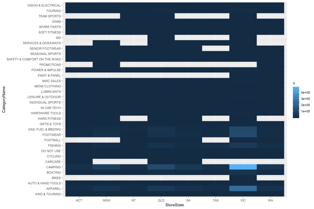
Due to the distribution of sales by product and state, it appears that any association rules we come up with will mainly be based on sales from VIC and QLD. Furthermore, as not all products were stocked/sold in all states, it is expected that the association rules will be limited to a very few number of products. However, since I have already embarked on this mode of analysis, let’s continue to see what we get.

由于按產品和州劃分的銷售額分布，看來我們提出的任何關聯規則都將主要基于VIC和QLD的銷售額。 此外，由于并非所有產品都在所有州都有庫存/出售，因此，預計關聯規則將限于極少數產品。 但是，由于我已經開始采用這種分析模式，所以讓我們繼續看看我們得到了什么。

We have two years worth of data, 2016 and 2017. So, I decided to compare the gross number of sales for the two years.

我們有2016年和2017年的兩年數據，因此，我決定比較這兩年的銷售總額。

Despite the higher number of transactions in 2016 (2.5 times more than 2017), mean gross sales were higher for 2017 than 2016. This seems quite counter-intuitive. So, I decided to dive into this deeper by looking at monthly sales.

盡管2016年交易數量增加(比2017年增加了2.5倍)，但2017年的平均銷售總額卻比2016年更高。這似乎是違反直覺的。 因此，我決定通過查看月度銷售來更深入地研究。

Year# of TransactionsMean Gross Sales ($)2016 1481922 $69.02017 593315 $86.0

交易年份1481922銷售總額($)2016 1481922 $ 69.02017 593315 $ 86.0

In 2016, the highest number of sales were recorded for January and March with steep declines in September to November and then an increase in December. However, transactions continued to decline in 2017 with an increase in December (Xmas season).

2016年，1月和3月的銷售記錄最高，9月至11月急劇下降，然后在12月上升。 但是，2017年交易繼續下降，12月(圣誕節季節)有所增加。

Deduction: As highest number of sales are for Camping, apparel and BBQ & Gas, it makes sense that sales for these products is high during the holiday season

扣除 ：由于露營，服裝和燒烤與天然氣的銷售量最高，因此在假期期間這些產品的銷售量很高

Recommendation to the retailer: May want to explore whether stores have sufficient stock for these products in Dec-Jan as they are the most popular.

給零售商的 建議 ：可能想探索商店中是否有足夠的庫存來存放這些產品，因為它們是最受歡迎的產品。

Deduction: Despite the steady decline in the number of transactions, mean gross sales continue to increase month on month with it being highest in Dec 2017. This indicates fewer customers that made purchases but made purchases of products of greater value.

扣除額 ：盡管交易數量穩步下降，但平均銷售總額仍逐月增加，在2017年12月達到最高。這表明購買商品的顧客減少了，但購買了更高價值的商品。

Recommendation: What can the retailer do to ensure there is a steady state of purchases throughout the year rather than an increasing trend with maximum number of purchases at the end of the year as the retailer is still paying overhead costs and employee salaries amongst other costs to run its stores?

建議 ：零售商應采取什么措施確保全年的采購狀況穩定，而不是在年底增加采購數量的增加趨勢，因為零售商仍需支付間接費用和員工薪金等開店？

購物籃分析/關聯規則 (Basket Analysis/Association Rules)

Let’s go back to our objective.

讓我們回到我們的目標。

Aim: To determine which products are customers likely to buy together in order to make recommendations for products

目的 ：確定客戶可能一起??購買哪些產品，以便為產品提供建議

I used the arules package and the read.transactions function to convert the dataset into a transaction object. A summary of this object gives the following output

我使用了arules包和read.transactions函數將數據集轉換為事務對象。 該對象的摘要提供以下輸出

## transactions as itemMatrix in sparse format with
##  1019952 rows (elements/itemsets/transactions) and
##  21209 columns (items) and a density of 9.531951e-05 
## 
## most frequent items:
##       GAS BOTTLE REFILL 9KG*       GAS BOTTLE REFILL 4KG* 
##                        30628                        11724 
## 6 PACK BUTANE - WILD COUNTRY SNAP HOOK ALUMINIUM GRIPWELL 
##                         9209                         7086 
## PEG TENT GALV 225X6.3MM P04G                      (Other) 
##                         6948                      1996372 
## 
## element (itemset/transaction) length distribution:
## sizes
##      1      2      3      4      5      6      7      8      9     10 
## 546138 234643 109888  55319  30185  16656   9878   6018   3716   2332 
##     11     12     13     14     15     16     17     18     19     20 
##   1611    993    751    490    353    237    157    140     99     88 
##     21     22     23     24     25     26     27     28     29     30 
##     53     48     28     31     20     13     12     15      8      1 
##     31     32     33     34     35     36     37     38     39     40 
##      4      2      4      3      4      1      4      2      1      4 
##     43     46 
##      1      1 
## 
##    Min. 1st Qu.  Median    Mean 3rd Qu.    Max. 
##   1.000   1.000   1.000   2.022   2.000  46.000 
## 
## includes extended item information - examples:
##   labels
## 1     10
## 2     11
## 3  11/12

Based on the output above, we can conclude the following.

根據上面的輸出，我們可以得出以下結論。

• There are 1019952 collections (baskets) of items and 21209 items.
  有1019952個項目(購物籃)和21209個項目。

• Density measures the percentage of non-zero cells in a sparse matrix. It is the total number of items that are purchased divided by the possible number of items in that matrix. You can calculate how many items were purchased by using density: 1019952212090.0000953 = 2,061,545

  密度衡量的是稀疏矩陣中非零單元格的百分比。 它是購買的商品總數除以該矩陣中的可能商品數。 您可以使用密度來計算購買了多少商品：1019952 21209 0.0000953 = 2,061,545

• Element (itemset/transaction) length distribution: This tells you you how many transactions are there for 1-itemset, for 2-itemset and so on. The first row is telling you the number of items and the second row is telling you the number of transactions.

  元素(項目集/事務)長度分布：告訴您1項目集，2項目集等的事務數量。 第一行告訴您項目的數量，第二行告訴您交易的數量。

• Majority of baskets (87%) consist of between 1 to 3 items.
  大部分籃子(87％)由1至3個物品組成。
• Minimum number of items in a basket = 1 and maximum = 46 (only one basket)
  一個籃子中的最小項目數= 1，最大= 46(僅一個籃子)
• Most popular items are gas bottle, gas bottle refill, gripwell, and peg tent.
  最受歡迎的物品是氣瓶，氣瓶筆芯，握把和固定帳篷。

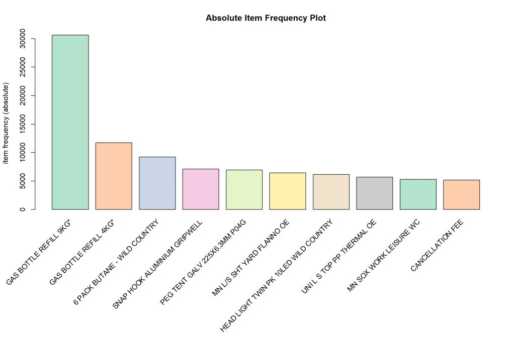
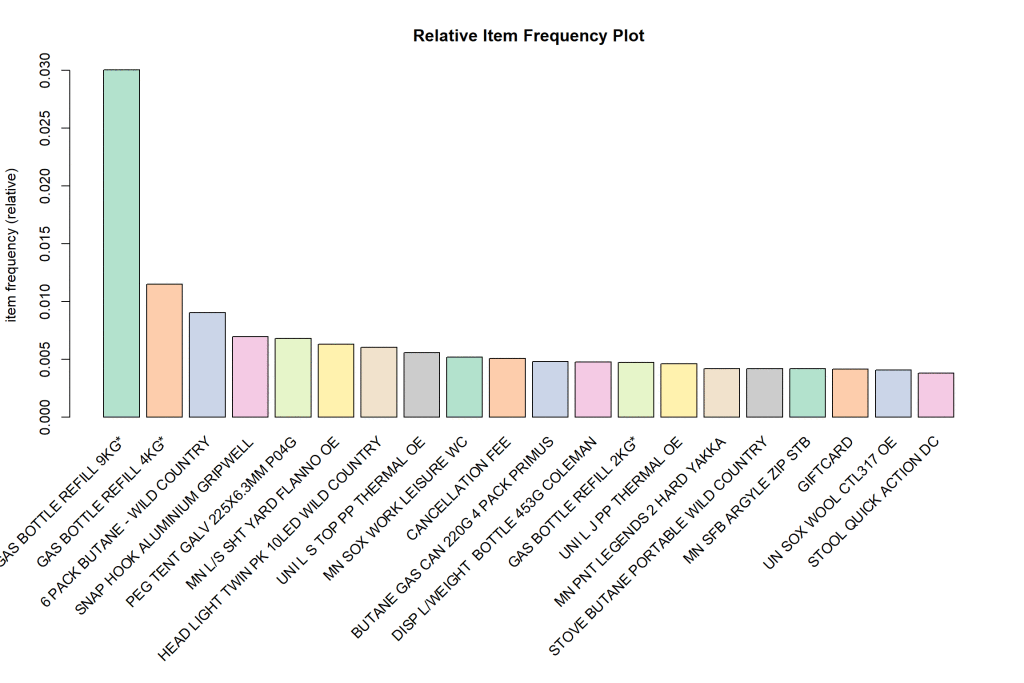
We can look at this information graphically via absolute frequency and relative frequency plots.

我們可以通過絕對頻率圖和相對頻率圖以圖形方式查看此信息。

Both plots are in descending order of frequency of purchase. The absolute frequency plot tells us that the highest number of sales are for gas related products. The relative frequency plot shows how the sales of the products that are close to each other in the bar chart are related to each other (i.e. relative). Thus, a recommendation that one can make to the retailer is to stock these products together in the store or send customers an EDM making recommendations for products that are related in the plot and have not yet been purchased by the customer.

兩種地塊均按購買頻率降序排列。 絕對頻率圖告訴我們，與氣體相關的產品銷量最高。 相對頻率圖顯示了條形圖中彼此接近的產品的銷售額如何相互關聯(即相對)。 因此，可以向零售商提出的建議是將這些產品一起存儲在商店中，或者向客戶發送EDM，以為該地塊中相關但尚未被客戶購買的產品提供建議。

The next step to do is to generate rules for our transaction object. The output is as follows.

下一步是為我們的交易對象生成規則。 輸出如下。

## Apriori
## 
## Parameter specification:
##  confidence minval smax arem  aval originalSupport maxtime support minlen
##         0.5    0.1    1 none FALSE            TRUE       5   0.001      1
##  maxlen target   ext
##      10  rules FALSE
## 
## Algorithmic control:
##  filter tree heap memopt load sort verbose
##     0.1 TRUE TRUE  FALSE TRUE    2    TRUE
## 
## Absolute minimum support count: 1019 
## 
## set item appearances ...[0 item(s)] done [0.00s].
## set transactions ...[21209 item(s), 1019952 transaction(s)] done [2.52s].
## sorting and recoding items ... [317 item(s)] done [0.04s].
## creating transaction tree ... done [0.84s].
## checking subsets of size 1 2 done [0.04s].
## writing ... [7 rule(s)] done [0.00s].
## creating S4 object  ... done [0.25s].

The above output shows us that 7 rules were generated.

上面的輸出向我們顯示了生成了7條規則。

Details of these rules are shown below.

這些規則的詳細信息如下所示。

## set of 7 rules
## 
## rule length distribution (lhs + rhs):sizes
## 2 
## 7 
## 
##    Min. 1st Qu.  Median    Mean 3rd Qu.    Max. 
##       2       2       2       2       2       2 
## 
## summary of quality measures:
##     support           confidence          lift            count     
##  Min.   :0.001128   Min.   :0.5458   Min.   : 26.30   Min.   :1150  
##  1st Qu.:0.001464   1st Qu.:0.6395   1st Qu.: 80.36   1st Qu.:1493  
##  Median :0.001650   Median :0.6634   Median :154.58   Median :1683  
##  Mean   :0.001652   Mean   :0.6759   Mean   :154.48   Mean   :1685  
##  3rd Qu.:0.001668   3rd Qu.:0.7265   3rd Qu.:245.30   3rd Qu.:1701  
##  Max.   :0.002524   Max.   :0.7898   Max.   :249.14   Max.   :2574  
## 
## mining info:
##  data ntransactions support confidence
##    tr       1019952   0.001        0.5

Now each of these rules have support, confidence, and lift values.

現在，每個規則都具有支持，信心和提升值。

Let’s start with support which is the proportion of transactions out of all transactions used to generate the rules (i.e. 1,019,952) that contain the two items together (i.e. 1190/1019952 = 0.0011 or 0.11%, where count is the number of transactions that contain the two items.

讓我們從支持開始，這是用于生成包含兩個項目的規則(即1,019,952)的所有交易中交易的比例(即1190/1019952 = 0.0011或0.11％，其中count是包含交易的數量)。兩個項目。

Confidence is the proportion of transactions where two items are bought together out of all transactions where one of the item is purchased. As these are apriori rules, the probability of buying item B is based on the purchase of item A.

置信度是在購買一件商品的所有交易中，同時購買兩項的交易所占的比例。 由于這些是先驗規則，因此購買項目B的概率基于對項目A的購買。

Mathematically, this looks like the following:

從數學上講，這類似于以下內容：

Confidence(A=>B) = P(A∩B) / P(A) = frequency(A,B) / frequency(A)

置信度(A?? => B)= P(A∩B)/ P(A)=頻率(A，B)/頻率(A)

In the results above, confidence values range from 54% to 79%.

在以上結果中，置信度范圍為54％至79％。

Probability of customers buying items together with confidence ranges from 54% to 79%, where buying item A has a positive effect on buying item B (as lift values are all greater than 1) .

客戶購買商品的概率連同置信度在54％到79％之間，其中購買商品A對購買商品B有積極影響(因為提升值都大于1)。

Note: When I ran the algorithm, I experimented with higher support and confidence values as if there is a greater number of transactions within the dataset where two items are bought together then the higher the confidence. However, when I ran the algorithm with 80% or more confidence, I obtained zero rules.

注意：當我運行算法時，我嘗試了更高的支持度和置信度值，好像在數據集中有兩個項目一起購買的交易數量較多時，置信度越高。 但是，當我以80％或更高的置信度運行算法時，我獲得了零規則。

This was expected due to the sparsity in data for frequent items where 1-item baskets are most common and the majority of purchased items related to camping or gas products.

可以預見，這是因為經常出現的物品(其中最常見的是1個項目的籃子)的數據稀疏，并且購買的大多數物品都與露營或天然氣產品有關。

Thus, the algorithm was run with the following parameters.

因此，該算法使用以下參數運行。

association.rules <- apriori(tr, parameter = list(supp=0.001, conf=0.5,maxlen=10))

Lift indicates how two items are correlated to each other. A positive lift value indicates that buying item A is likely to result in a purchase of item B. Mathematically, lift is calculated as follows.

提升指示兩個項目如何相互關聯。 正提升值表示購買商品A可能導致購買商品B。在數學上， 提升計算如下。

Lift(A=>B) = Support / (Supp(A) * Supp(B) )

提升(A => B)=支撐/(支持(A)*支持(B))

All our rules have positive lift values indicating that buying item A is likely to lead to a purchase of item B.

我們所有的規則都具有正提升值，表明購買商品A可能導致購買商品B。

規則檢查 (Rules inspection)

Let’s now inspect the rules.

現在讓我們檢查規則。

lhs    rhs   support confidence      lift count
## [1] {GAS BOTTLE 9KG POL CODE 2 DC} => {GAS BOTTLE REFILL 9KG*}       0.001650078  0.7897701  26.30036  1683
## [2] {WEBER BABY Q (Q1000) ROASTING TRIVET} => {WEBER BABY Q CONVECTION TRAY} 0.001127504  0.6526674 241.45428  1150
## [3] {GAS BOTTLE 2KG CODE 4 DC}             => {GAS BOTTLE REFILL 2KG*}       0.001344181  0.7308102 154.58137  1371
## [4] {GAS BOTTLE 4KG POL CODE 2 DC}         => {GAS BOTTLE REFILL 4KG*}       0.001583408  0.7222719  62.83544  1615
## [5] {YTH L J PP THERMAL OE}                => {YTH LS TOP PP THERMAL OE}     0.001667726  0.6634165 249.13587  1701
## [6] {YTH LS TOP PP THERMAL OE}             => {YTH L J PP THERMAL OE}        0.001667726  0.6262887 249.13587  1701
## [7] {UNI L J PP THERMAL OE}                => {UNI L S TOP PP THERMAL OE}    0.002523648  0.5458015  97.88840  2574

Interpretation of the first rule is as follows:

第一條規則的解釋如下：

If a customer buys the 9kg gas bottle, there is a 79% chance that customer will also buy its refill. This is identified for 1,683 transactions in the dataset.

如果客戶購買了9公斤的氣瓶，則客戶也有79％的機會購買其補充裝。 在數據集中為 1,683個事務確定了這一點 。

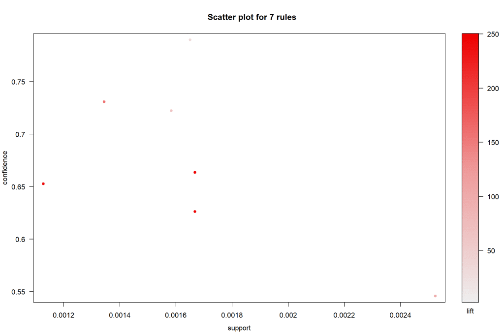
Now, let’s look at these plots visually.

現在，讓我們直觀地查看這些圖。

All rules have a confidence value greater than 0.5 with lift ranging from 26 to 249.

所有規則的置信度值都大于0.5，提升范圍為26至249。

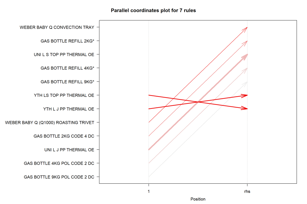
The Parallel coordinates plot for the seven rules shows how the purchase of one product influences the purchase of another product. RHS is the item we propose the customer buy. For LHS, 2 is the most recent addition to the basket and 1 is the item that the customer previously purchased.

七個規則的平行坐標圖顯示了一種產品的購買如何影響另一種產品的購買。 RHS是我們建議客戶購買的物品。 對于LHS，購物籃中最新添加了2個，客戶先前購買的商品是1個。

Looking at the first arrow we can see that if a customer has Weber Baby (Q1000) roasting trivet in their basket, then they are likely to purchase weber babgy q convection tray.

查看第一個箭頭，我們可以看到，如果客戶的購物籃中裝有Weber Baby(Q1000)烤三角架，那么他們很可能會購買Weber babgy q對流托盤。

The below plots would be more useful if we could visualize more than 2-itemset baskets.

如果我們可以可視化超過2個項目的購物籃，則以下圖表將更加有用。

結語 (Wrapping up)

You have now learnt how to make recommendations to customers based on which items are most frequently purchased together based on apriori rules. However, some important things to note about this analysis.

現在，您已經了解了如何根據先驗規則，根據最常一起購買的商品向客戶提出建議。 但是，有關此分析的一些重要注意事項。

• The most popular/frequent items have confounded the analysis to some extent where it appears that we can only make recommendations with respect to only seven association rules with confidence. This is due to the uneven distribution of the number of items by frequency in the basket.
  最受歡迎/最常見的項目在某種程度上使分析變得混亂，因為我們似乎只能自信地針對七個關聯規則提出建議。 這是由于籃子中物品數量按頻率的不均勻分布所致。
• Customer segmentation may be another approach for this dataset where customers are grouped by spend (SalesGross), product type (i.e. CategoryCode), StateStore, and time of sale (i.e. Month/Year). However, it would be useful to have more features on customers to do this effectively.
  客戶細分可能是此數據集的另一種方法，其中按支出(SalesGross)，產品類型(即CategoryCode)，StateStore和銷售時間(即月/年)對客戶進行分組。 但是，為客戶提供更多功能以有效地執行此操作將很有用。

Code and dataset: https://github.com/shedoesdatascience/basketanalysis

代碼和數據集： https : //github.com/shedoesdatascience/basketanalysis