For detailed implementation in python check my GitHub repository.

有關在python中的詳細實現，請查看我的GitHub存儲庫。

介紹 (Introduction)

Some machine learning model like linear and logistic regression assumes a Gaussian distribution or normal distribution. One of the first steps of statistical analysis of your data is therefore to check the distribution of the data.

某些機器學習模型(例如線性和邏輯回歸)采用高斯分布或正態分布。 因此，對數據進行統計分析的第一步就是檢查數據的分布。

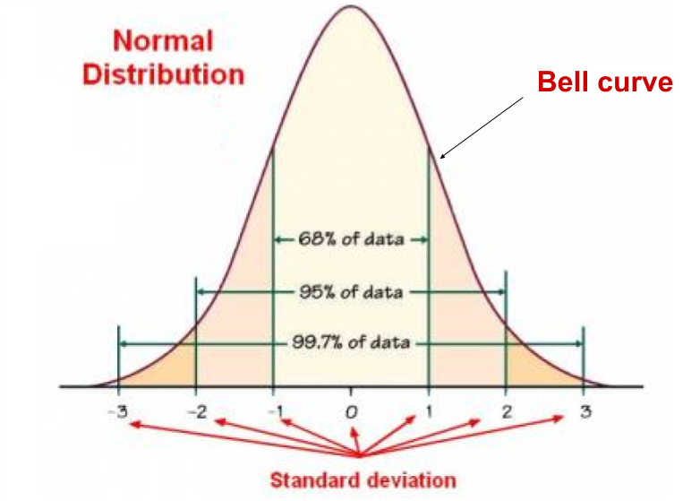
The familiar bell curve shows a normal distribution.

熟悉的鐘形曲線顯示正態分布。

If your data has a Gaussian distribution, the machine learning methods are powerful and well understood.

如果您的數據具有高斯分布，則機器學習方法功能強大且易于理解。

Most of the data scientists claim they are getting more accurate results when they transform the predictor variables.

大多數數據科學家聲稱，他們在轉換預測變量時會獲得更準確的結果。

To transform data, you perform a mathematical operation on each observation, then use these transformed data in our model.

要轉換數據，您需要對每個觀測值執行數學運算，然后在我們的模型中使用這些轉換后的數據。

為什么我們需要正態分布？ (Why do we need a normal distribution?)

If a method that assumes a Gaussian distribution, and your data was drawn from a different distribution other then normal distribution, then the findings may be misleading or plain wrong.

如果采用假定高斯分布的方法，并且您的數據是從不同于正態分布的其他分布中提取的，則發現可能會產生誤導或明顯錯誤。

It is possible that your data does not look Gaussian or fails a normality test, but can be transformed to make it fit a Gaussian distribution.

您的數據看起來可能不是高斯或未通過正態性檢驗，但可以進行轉換以使其適合高斯分布。

轉換類型 (Type of transformation)

1. Log Transformation
   日志轉換
2. Reciprocal Transformation
   相互轉換
3. Square-Root Transformation
   平方根變換
4. Cube root Transformation
   立方根轉換
5. Exponential Transformation
   指數變換
6. Box-Cox Transformation
   Box-Cox轉換
7. Yeo-Johnson Transformation
   楊約翰遜變換

可視化并檢查分布 (Visualize and Checks distribution)

We can create plots of the data to check whether it is Gaussian or not.

我們可以創建數據圖以檢查其是否為高斯。

We will look at two common methods for visually inspecting a dataset to check if it was drawn from a Gaussian distribution.

我們將看兩種常見的方法，以可視方式檢查數據集以檢查它是否是從高斯分布中提取的。

1. Histogram
   直方圖
2. Quantile-Quantile plot (Q-Q plot)
   分位數圖(QQ圖)

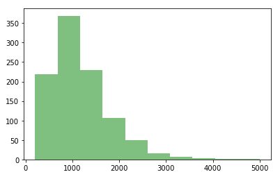
1.直方圖 (1. Histogram)

A histogram is a plot that lets you discover, and show, the underlying frequency distribution (shape) of a set of continuous data. This allows the inspection of the data for its underlying distribution (e.g., normal distribution), outliers, skewness, etc.

直方圖是一種圖表，可讓您發現并顯示一組連續數據的基礎頻率分布(形狀)。 這允許檢查數據的基本分布(例如，正態分布)，離群值，偏度等。

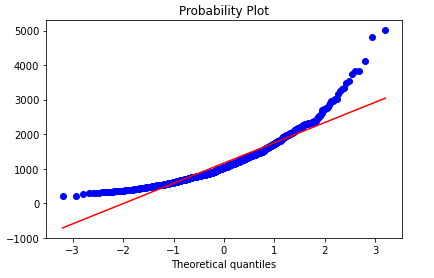
2. QQ圖 (2. Q-Q Plot)

The Q-Q plot, or quantile-quantile, are plots of two quantiles against each other. A quantile is a fraction where certain values fall below that quantile.

QQ圖(或分位數)是兩個分位數彼此相對的圖。 分位數是某些值低于該分位數的分數。

For example, the median is a quantile where 50% of the data fall below that point and 50% lie above it.

例如，中位數是一個分位數，其中50％的數據低于該點，而50％的數據位于該點之上。

The purpose of Q Q plots is to find out if two sets of data come from the same distribution. A 45-degree angle is plotted on the Q Q plot; if the two data sets come from a common distribution, the points will fall on that reference line.

QQ圖的目的是找出兩組數據是否來自同一分布。 QQ圖上繪制了45度角； 如果兩個數據集來自同一分布，則這些點將落在該參考線上。

數據 (Data)

We will use randomly generated data in this article to demonstrate all techniques.

我們將在本文中使用隨機生成的數據來演示所有技術。

# generate a univariate data sample
np.random.seed(142)
datas = sorted(stats.lognorm.rvs(s=0.5, loc=1, scale=1000, size=1000))# convert to dataframe
data = pd.DataFrame(datas, columns=['values'])#

生成圖的方法 (Method to generate a graph)

After we transform our data each time we will call this method to generate a graph.

每次轉換數據后，我們將調用此方法來生成圖形。

def gen_graph(value):
    plt.figure(figsize=(15,5))
    plt.subplot(1, 2, 1)
    plt.hist(value, color='g', alpha=0.5)    plt.subplot(1, 2, 2)
    stats.probplot(value, dist="norm", plot=plt)    plt.show()

轉換前可視化數據 (visualize data before transformation)

gen_graph(data['values'])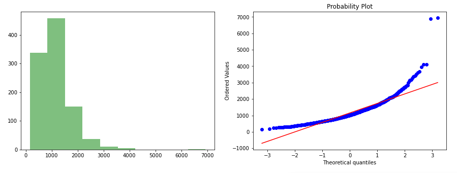

1.日志轉換 (1. Log Transformation)

Log or Logarithmic transformation is a data transformation method in which we replace each variable x with a log(x). When our original continuous data do not follow the bell curve, we can log transform this data to make it “normal”.

對數或對數轉換是一種數據轉換方法，其中我們將每個變量x替換為log(x)。 當我們的原始連續數據不遵循鐘形曲線時，我們可以對數據進行對數轉換以使其“正常”。

data_log = np.log(data['values'])gen_graph(data_log)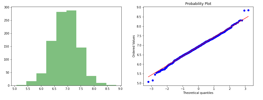

2.相互轉化 (2. Reciprocal Transformation)

The reciprocal transformation is defined as the transformation of x to 1/x. The transformation has a dramatic effect on the shape of the distribution, reversing the order of values with the same sign. The transformation can only be used for non-zero values.

互逆變換定義為x到1 / x的變換。 變換對分布的形狀產生了巨大影響，顛倒了具有相同符號的值的順序。 轉換只能用于非零值。

data_rec = np.reciprocal(data['values'])# ordata_rec_2 = 1/data['values']gen_graph(data_rec)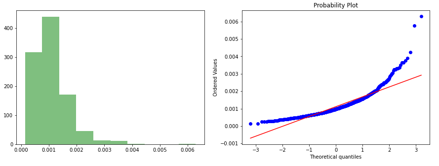

3.平方根變換 (3. Square-Root Transformation)

The square root of your variables, i.e. x → x(1/2) = sqrt(x). This will have a moderate effect on the distribution and usually works for data with non-constant variance. However, it is considered to be weaker than logarithmic or cube root transforms.

變量的平方根，即x→x(1/2)= sqrt(x)。 這將對分布產生適度的影響，并且通常適用于具有非恒定方差的數據。 但是，它被認為比對數或立方根轉換要弱。

data_square = np.sqrt(data['values'])# or 
data_square_2 = (data)**(1/2)gen_graph(data_square)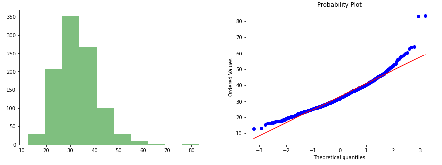

4.多維數據集根轉換 (4. Cube root Transformation)

The cube root transformation involves converting x to x^(1/3).

立方根轉換涉及將x轉換為x ^(1/3)。

It is useful for reducing the right skewness. This is a fairly strong transformation with a substantial effect on the distribution shape but is weaker than the logarithm. It can be applied to negative and zero values too. Negatively skewed data.

這對于減少正確的偏斜很有用。 這是一個相當強的變換，對分布形狀有很大影響，但比對數弱。 它也可以應用于負值和零值。 負偏斜數據。

data_cube = np.cbrt(data['values'])gen_graph(data_cube)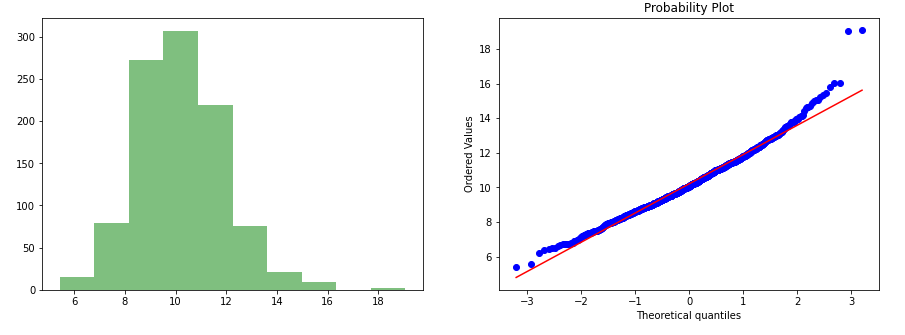

5.指數變換 (5. Exponential Transformation)

An exponential transformation provides a useful alternative to Box and Cox’s, one parameter power transformation, and has the advantage of allowing negative data values.

指數變換是Box和Cox變換的一種有用的替代方法，它是一種參數冪變換，并且具有允許負數據值的優點。

It has been found in particular that this transformation is quite effective at turning skew unimodal distribution into nearly symmetric normal like distribution.

特別地，已經發現該變換在將偏斜單峰分布轉變成近似對稱的正態分布方面非常有效。

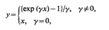
data_expo =  data['values'] ** (1/5)gen_graph(data_expo)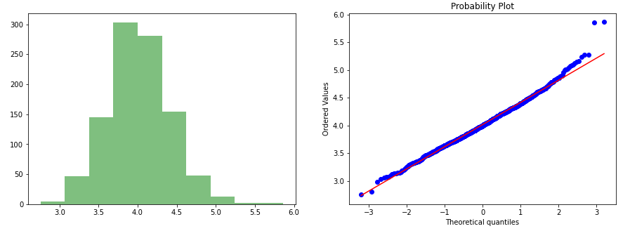

6. Box-Cox轉換 (6. Box-Cox Transformation)

At the core of the Box-Cox transformation is an exponent, lambda (λ), which varies from -5 to 5.

Box-Cox變換的核心是指數lambda(λ)，從-5到5不等。

All values of λ are considered, and the optimal value for your data is selected; The “optimal value” is the one which results in the best approximation of a normal distribution curve. The transformation of Y has the form:

考慮所有λ值，并選擇數據的最佳值； “最佳值”是導致正態分布曲線最佳近似的值。 Y的轉換形式為：

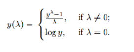
data_boxcox, a = stats.boxcox(data['values'])gen_graph(data_boxcox)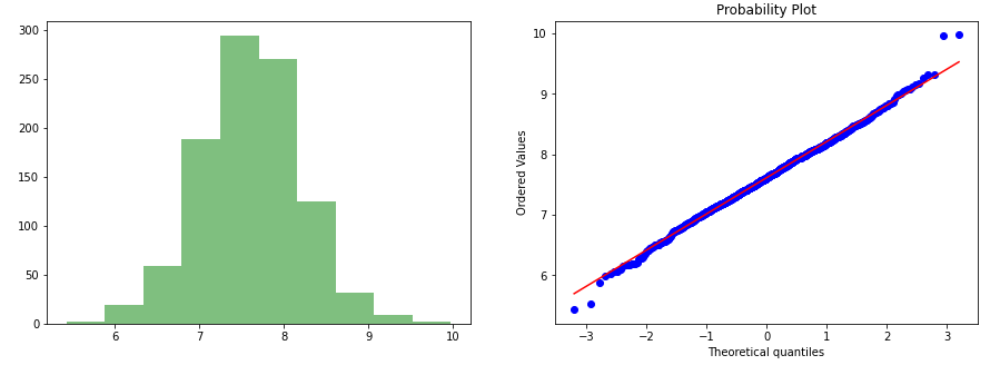

7.楊約翰遜轉型 (7. Yeo-Johnson Transformation)

This is one of the older transformation technique which is very similar to Box-cox transformation but does not require the values to be strictly positive.This transformation is also having the ability to make the distribution more symmetric.

這是較舊的變換技術之一，與Box-cox變換非常相似，但不需要嚴格將值設為正數。此變換還具有使分布更加對稱的能力。

data_yeo, a = stats.yeojohnson(data['values'])gen_graph(data_yeo)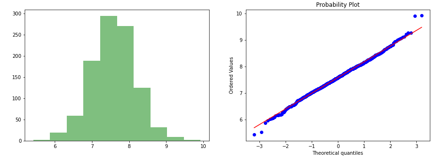

結論 (Conclusion)

In this article, we have seen the different types of transformations to normalized the distribution of data. Box-cox and log transformation is one of the best transformation technique that gives us a good result.

在本文中，我們已經看到了不同類型的轉換以標準化數據的分布。 Box-cox和log轉換是最好的轉換技術之一，可以為我們帶來良好的效果。

Hope you like this article.

希望您喜歡這篇文章。

Follow me for more such interesting article

跟隨我獲得更多如此有趣的文章

Please clap and show your appreciation :)

請鼓掌并表示感謝：)

Thanks for reading. 😃

謝謝閱讀。 😃