機器學習啤酒數據集

Artificial neural networks (ANNs), usually simply called neural networks (NNs), are computing systems vaguely inspired by the biological neural networks that constitute animal brains.

人工神經網絡(ANN)通常簡稱為神經網絡(NNs)，是由構成動物大腦的生物神經網絡模糊地啟發了計算系統。

An ANN is based on a collection of connected units or nodes called artificial neurons, which loosely model the neurons in a biological brain. Each connection, like the synapses in a biological brain, can transmit a signal to other neurons. An artificial neuron that receives a signal then processes it and can signal neurons connected to it. The “signal” at a connection is a real number, and the output of each neuron is computed by some non-linear function of the sum of its inputs. The connections are called edges. Neurons and edges typically have a weight that adjusts as learning proceeds. The weight increases or decreases the strength of the signal at a connection. Neurons may have a threshold such that a signal is sent only if the aggregate signal crosses that threshold. Typically, neurons are aggregated into layers. Different layers may perform different transformations on their inputs. Signals travel from the first layer (the input layer), to the last layer (the output layer), possibly after traversing the layers multiple times.

人工神經網絡基于稱為人工神經元的連接單元或節點的集合，這些單元或節點可以對生物腦中的神經元進行松散建模。每個連接都像生物大腦中的突觸一樣，可以將信號傳輸到其他神經元。接收信號的人工神經元隨后對其進行處理，并可以向與之相連的神經元發出信號。連接處的“信號”是實數，每個神經元的輸出通過其輸入之和的某些非線性函數來計算。這些連接稱為邊。神經元和邊緣通常具有隨著學習的進行而調整的權重。權重增加或減小連接處信號的強度。神經元可以具有閾值，使得僅當總信號超過該閾值時才發送信號。通常，神經元聚集成層。不同的層可以對它們的輸入執行不同的變換。信號可能從第一層(輸入層)傳播到最后一層(輸出層)，可能是在多次遍歷這些層之后。

Neural networks learn (or are trained) by processing examples, each of which contains a known “input” and “result,” forming probability-weighted associations between the two, which are stored within the data structure of the net itself. The training of a neural network from a given example is usually conducted by determining the difference between the processed output of the network (often a prediction) and a target output. This is the error. The network then adjusts it’s weighted associations according to a learning rule and using this error value. Successive adjustments will cause the neural network to produce output which is increasingly similar to the target output. After a sufficient number of these adjustments the training can be terminated based upon certain criteria. This is known as [[supervised learning]].

神經網絡通過處理示例來學習(或訓練)，每個示例都包含一個已知的“輸入”和“結果”，形成兩者之間的概率加權關聯，這些關聯存儲在網絡本身的數據結構中。給定示例中的神經網絡訓練通常是通過確定網絡的處理輸出(通常是預測)與目標輸出之間的差異來進行的。這是錯誤。然后，網絡根據學習規則并使用此錯誤值來調整其加權關聯。連續的調整將導致神經網絡產生越來越類似于目標輸出的輸出。在進行了足夠數量的這些調整后，可以基于某些標準終止訓練。這稱為[[監督學習]]。

開始干活 (Let’s work)

安裝套件 (Install Packages)

packages <- c("xts","zoo","PerformanceAnalytics", "GGally", "ggplot2", "ellipse", "plotly")
newpack  = packages[!(packages %in% installed.packages()[,"Package"])]
if(length(newpack)) install.packages(newpack)
a=lapply(packages, library, character.only=TRUE)

加載數據集 (Load dataset)

beer <- read.csv("MyData.csv")
head(beer)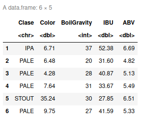

summary(beer)Clase               Color        BoilGravity        IBU        
 Length:1000        Min.   : 1.99   Min.   : 1.0   Min.   :  0.00  
 Class :character   1st Qu.: 5.83   1st Qu.:27.0   1st Qu.: 32.90  
 Mode  :character   Median : 7.79   Median :33.0   Median : 47.90  
                    Mean   :13.45   Mean   :33.8   Mean   : 51.97  
                    3rd Qu.:12.57   3rd Qu.:39.0   3rd Qu.: 67.77  
                    Max.   :50.00   Max.   :90.0   Max.   :144.53  
      ABV        
 Min.   : 2.390  
 1st Qu.: 5.240  
 Median : 5.990  
 Mean   : 6.093  
 3rd Qu.: 6.810  
 Max.   :10.380

虹膜數據集的可視化 (Visualization of Iris Data Set)

You can also embed plots, for example:

您還可以嵌入圖，例如：

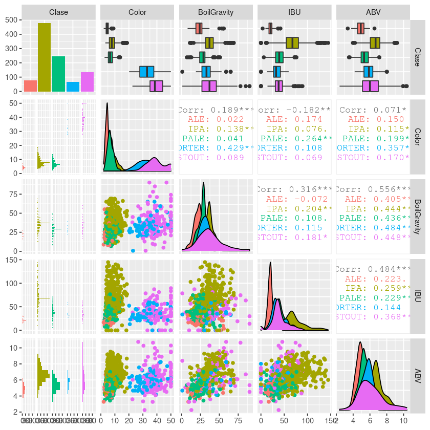
pairs(beer[2:5], 
      main = "Craft Beer Data -- 5 types",
      pch = 21, bg = c("red", "green", "blue", "orange", "yellow"))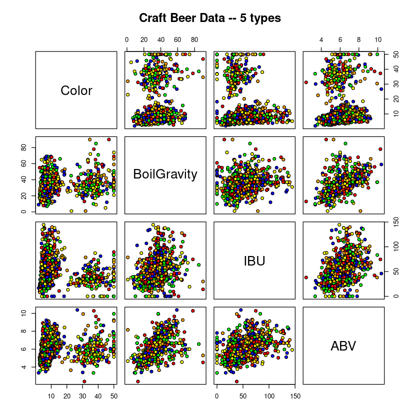

library(GGally)
pm <- ggpairs(beer,lower=list(combo=wrap("facethist",  
binwidth=0.5)),title="Craft Beer", mapping=aes(color=Clase))
pm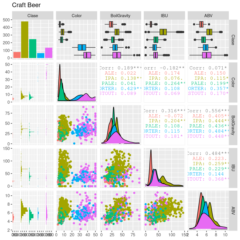

library(PerformanceAnalytics)
chart.Correlation2 <- function (R, histogram = TRUE, method = NULL, ...)
    {
        x = checkData(R, method = "matrix")
        if (is.null(method)) #modified
            method = 'pearson'
  
        use.method <- method #added
        panel.cor <- function(x, y, digits = 2, prefix = "", 
                              use = "pairwise.complete.obs", 
                              method = use.method, cex.cor, ...) 
        { #modified
        usr <- par("usr")
        on.exit(par(usr))
        par(usr = c(0, 1, 0, 1))
        r <- cor(x, y, use = use, method = method)
        txt <- format(c(r, 0.123456789), digits = digits)[1]
        txt <- paste(prefix, txt, sep = "")
        if (missing(cex.cor)) 
            cex <- 0.8/strwidth(txt)
        test <- cor.test(as.numeric(x), as.numeric(y), method = method)
        Signif <- symnum(test$p.value, corr = FALSE, na = FALSE, 
                         cutpoints = c(0, 0.001, 0.01, 0.05, 0.1, 1),
                         symbols = c("***","**", "*", ".", " "))
        text(0.5, 0.5, txt, cex = cex * (abs(r) + 0.3)/1.3)
        text(0.8, 0.8, Signif, cex = cex, col = 2)
        }
    f <- function(t)
        {
        dnorm(t, mean = mean(x), sd = sd.xts(x))
        }
    dotargs <- list(...)
    dotargs$method <- NULL
    rm(method)
    hist.panel = function(x, ... = NULL) 
        {
        par(new = TRUE)
        hist(x, col = "light gray", probability = TRUE, axes = FALSE, 
             main = "", breaks = "FD")
        lines(density(x, na.rm = TRUE), col = "red", lwd = 1)
        rug(x)
        }
    if (histogram) 
        pairs(x, gap = 0, lower.panel = panel.smooth, 
              upper.panel = panel.cor, diag.panel = hist.panel)
    else pairs(x, gap = 0, lower.panel = panel.smooth, upper.panel = panel.cor)
    }
#if method option not set default is 'pearson'
chart.Correlation2(beer[,2:5], histogram=TRUE, pch="21")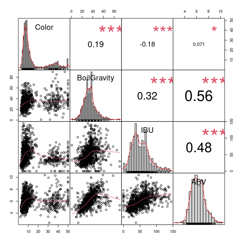

library(plotly)
pm <- GGally::ggpairs(beer, aes(color = Clase), lower=list(combo=wrap("facethist",  
binwidth=0.5)))
class(pm)
pm

‘gg’
'gg'
‘ggmatrix’
'ggmatrix'

建立和訓練啤酒數據神經網絡 (Setup and Train the Neural Network for Beer Data)

Neural Network emulates how the human brain works by having a network of neurons that are interconnected and sending stimulating signal to each other.

神經網絡通過使相互連接的神經元網絡相互發送刺激信號來模擬人腦的工作方式。

In the Neural Network model, each neuron is equivalent to a logistic regression unit. Neurons are organized in multiple layers where every neuron at layer i connects out to every neuron at layer i+1 and nothing else.

在神經網絡模型中，每個神經元都等效于邏輯回歸單元。神經元是多層組織的，其中第i層的每個神經元都與第i + 1層的每個神經元相連。

The tuning parameters in Neural network includes the number of hidden layers, number of neurons in each layer, as well as the learning rate.

神經網絡中的調整參數包括隱藏層數，每層神經元數以及學習率。

There are no fixed rules to set these parameters and depends a lot in the problem domain. My default choice is to use a single hidden layer and set the number of neurons to be the same as the input variables. The number of neurons at the output layer depends on how many binary outputs need to be learned. In a classification problem, this is typically the number of possible values at the output category.

沒有固定的規則來設置這些參數，并且在問題域中有很大關系。我的默認選擇是使用單個隱藏層，并將神經元數量設置為與輸入變量相同。輸出層神經元的數量取決于需要學習多少個二進制輸出。在分類問題中，這通常是輸出類別中可能值的數量。

The learning happens via an iterative feedback mechanism where the error of training data output is used to adjusted the corresponding weights of input. This adjustment will be propagated back to previous layers and the learning algorithm is known as back-propagation.

通過迭代反饋機制進行學習，在該機制中，訓練數據輸出的錯誤用于調整輸入的相應權重。此調整將傳播回先前的層，學習算法稱為反向傳播。

library(neuralnet)beer <- beer%>%
    select("IBU","ABV","Color","BoilGravity","Clase")
head(beer)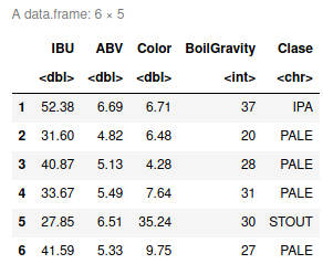

# Binarize the categorical output
beer <- cbind(beer, beer$Clase == 'ALE')
beer <- cbind(beer, beer$Clase == 'IPA')
beer <- cbind(beer, beer$Clase == 'PALE')
beer <- cbind(beer, beer$Clase == 'STOUT')
beer <- cbind(beer, beer$Clase == 'PORTER')
names(beer)[6] <- 'ALE'
names(beer)[7] <- 'IPA'
names(beer)[8] <- 'PALE'
names(beer)[9] <- 'STOUT'
names(beer)[10] <- 'PORTER'
head(beer)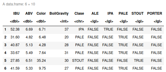

set.seed(101)
beer.train.idx <- sample(x = nrow(beer), size = nrow(beer)*0.5)
beer.train <- beer[beer.train.idx,]
beer.valid <- beer[-beer.train.idx,]

啤酒數據神經網絡的可視化 (Visulization of the Neural Network on Beer Data)

Here is the plot of the Neural network we learn

這是我們學習的神經網絡圖

Neural network is very good at learning non-linear function and also multiple outputs can be learnt at the same time. However, the training time is relatively long and it is also susceptible to local minimum traps. This can be mitigated by doing multiple rounds and pick the best learned model.

神經網絡非常擅長學習非線性函數，并且可以同時學習多個輸出。但是，訓練時間相對較長，并且也容易受到局部最小陷阱的影響。可以通過多次嘗試并選擇最佳的學習模型來緩解這種情況。

nn <- neuralnet(ALE+IPA+PALE+STOUT+PORTER ~ IBU+ABV+Color+BoilGravity, data=beer.train, hidden=c(5))plot(nn, rep = "best")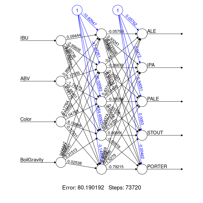

結果 (Result)

beer.prediction <- compute(nn, beer.valid[-5:-10])
idx <- apply(beer.prediction$net.result, 1, which.max)
predicted <- c('ALE','IPA', 'PALE', 'STOUT', 'PORTER')[idx]
table(predicted, beer.valid$Clase)predicted ALE IPA PALE PORTER STOUT
    ALE    17   3   12      0     0
    IPA     1 203   21      0     2
    PALE   29  26   84      1     0
    STOUT   0   4    0     30    67

Accuracy of model is calculated as follows

模型的精度計算如下

((17+203+84+0+67)/nrow(beer.valid))*100

74.2

# nn$result.matrixstr(nn)List of 14
 $ call               : language neuralnet(formula = ALE + IPA + PALE + STOUT + PORTER ~ IBU + ABV + Color +      BoilGravity, data = beer.train, hidden = c(5))
 $ response           : logi [1:500, 1:5] FALSE FALSE FALSE FALSE FALSE FALSE ...
  ..- attr(*, "dimnames")=List of 2
  .. ..$ : chr [1:500] "841" "825" "430" "95" ...
  .. ..$ : chr [1:5] "ALE" "IPA" "PALE" "STOUT" ...
 $ covariate          : num [1:500, 1:4] 62.3 27.1 39 72.3 67.8 ...
  ..- attr(*, "dimnames")=List of 2
  .. ..$ : chr [1:500] "841" "825" "430" "95" ...
  .. ..$ : chr [1:4] "IBU" "ABV" "Color" "BoilGravity"
 $ model.list         :List of 2
  ..$ response : chr [1:5] "ALE" "IPA" "PALE" "STOUT" ...
  ..$ variables: chr [1:4] "IBU" "ABV" "Color" "BoilGravity"
 $ err.fct            :function (x, y)  
  ..- attr(*, "type")= chr "sse"
 $ act.fct            :function (x)  
  ..- attr(*, "type")= chr "logistic"
 $ linear.output      : logi TRUE
 $ data               :'data.frame':	500 obs. of  10 variables:
  ..$ IBU        : num [1:500] 62.3 27.1 39 72.3 67.8 ...
  ..$ ABV        : num [1:500] 5.9 5.07 6.57 5.7 6.86 5.21 4.22 5.57 5.76 7.76 ...
  ..$ Color      : num [1:500] 5.61 32.07 39.92 9.62 8.29 ...
  ..$ BoilGravity: int [1:500] 37 25 40 37 31 28 19 27 30 44 ...
  ..$ Clase      : chr [1:500] "IPA" "PORTER" "STOUT" "PALE" ...
  ..$ ALE        : logi [1:500] FALSE FALSE FALSE FALSE FALSE FALSE ...
  ..$ IPA        : logi [1:500] TRUE FALSE FALSE FALSE TRUE FALSE ...
  ..$ PALE       : logi [1:500] FALSE FALSE FALSE TRUE FALSE TRUE ...
  ..$ STOUT      : logi [1:500] FALSE FALSE TRUE FALSE FALSE FALSE ...
  ..$ PORTER     : logi [1:500] FALSE TRUE FALSE FALSE FALSE FALSE ...
 $ exclude            : NULL
 $ net.result         :List of 1
  ..$ : num [1:500, 1:5] 0.00942 0.01859 0.01845 0.00916 0.00478 ...
  .. ..- attr(*, "dimnames")=List of 2
  .. .. ..$ : chr [1:500] "841" "825" "430" "95" ...
  .. .. ..$ : NULL
 $ weights            :List of 1
  ..$ :List of 2
  .. ..$ : num [1:5, 1:5] -10.8295 0.0944 0.9985 -0.1776 0.0445 ...
  .. ..$ : num [1:6, 1:5] 0.0576 -0.058 -0.4324 0.4371 -0.0437 ...
 $ generalized.weights:List of 1
  ..$ : num [1:500, 1:20] -0.08239 -0.000124 -0.000822 -0.082905 -0.093232 ...
  .. ..- attr(*, "dimnames")=List of 2
  .. .. ..$ : chr [1:500] "841" "825" "430" "95" ...
  .. .. ..$ : NULL
 $ startweights       :List of 1
  ..$ :List of 2
  .. ..$ : num [1:5, 1:5] -0.5 1.832 -0.329 0.261 -1.112 ...
  .. ..$ : num [1:6, 1:5] 0.341 1.107 0.689 0.471 -1.64 ...
 $ result.matrix      : num [1:58, 1] 8.02e+01 8.76e-03 7.37e+04 -1.08e+01 9.44e-02 ...
  ..- attr(*, "dimnames")=List of 2
  .. ..$ : chr [1:58] "error" "reached.threshold" "steps" "Intercept.to.1layhid1" ...
  .. ..$ : NULL
 - attr(*, "class")= chr "nn"beer.net <- neuralnet(ALE+IPA+PALE+STOUT+PORTER ~ IBU+ABV+Color+BoilGravity, 
                      data=beer.train, hidden=c(5),  err.fct = "ce", 
                      linear.output = F, lifesign = "minimal", 
                      threshold = 0.1)hidden: 5    thresh: 0.1    rep: 1/1    steps: 
  86036
	error: 431.94881
	time: 24.02 secsplot(beer.net, rep="best")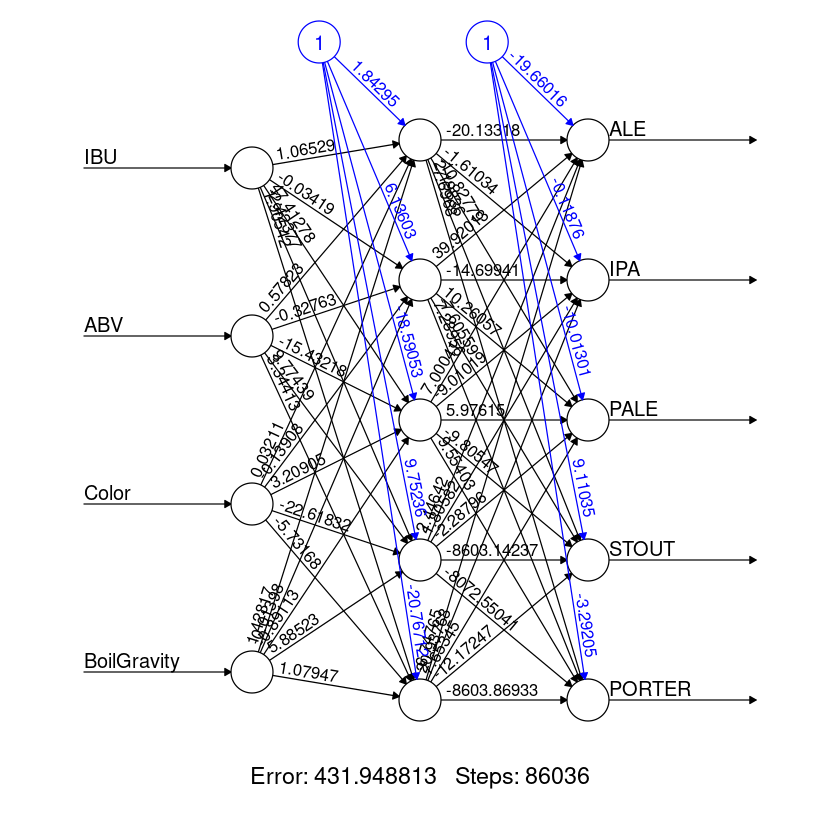

預測結果 (Predicting Result)

beer.prediction <- compute(beer.net, beer.valid[-5:-10])
idx <- apply(beer.prediction$net.result, 1, which.max)
predicted <- c('ALE','IPA', 'PALE', 'STOUT', 'PORTER')[idx]
table(predicted, beer.valid$Clase)predicted ALE IPA PALE PORTER STOUT
   ALE     26   4    9      0     0
   IPA      0 197   30      1     3
   PALE    21  33   78      0     0
   PORTER   0   1    0     10     6
   STOUT    0   1    0     20    60

Accuracy of model is calculated as follows

模型的精度計算如下

((26+197+78+10+60)/nrow(beer.valid))*100

74.2

結論 (Conclusion)

As you can see the accuracy is equal!

如您所見，精度是相等的！

I hope it will help you to develop your training.

我希望它能幫助您發展培訓。

永不放棄！ (Never give up!)

See you in Linkedin!

在Linkedin上見！

翻譯自: https://medium.com/@zumaia/neural-network-on-beer-dataset-55d62a0e7c32

機器學習啤酒數據集

本文來自互聯網用戶投稿，該文觀點僅代表作者本人，不代表本站立場。本站僅提供信息存儲空間服務，不擁有所有權，不承擔相關法律責任。
如若轉載，請注明出處：http://www.pswp.cn/news/388491.shtml
繁體地址，請注明出處：http://hk.pswp.cn/news/388491.shtml
英文地址，請注明出處：http://en.pswp.cn/news/388491.shtml

如若內容造成侵權/違法違規/事實不符，請聯系多彩編程網進行投訴反饋email:809451989@qq.com，一經查實，立即刪除！