Linear Regression is the Supervised Machine Learning Algorithm that predicts continuous value outputs. In Linear Regression we generally follow three steps to predict the output.

線性回歸是一種監督機器學習算法，可預測連續值輸出。 在線性回歸中，我們通常遵循三個步驟來預測輸出。

1. Use Least-Square to fit a line to data

1.使用最小二乘法將一條線擬合到數據

2. Calculate R-Squared

2.計算R平方

3. Calculate p-value

3.計算p值

使一條線適合數據 (Fitting a line to a data)

There can be many lines that can be fitted within the data, but we have to consider only that one which has very less error.

數據中可以包含許多行，但是我們只需要考慮誤差很小的那一行。

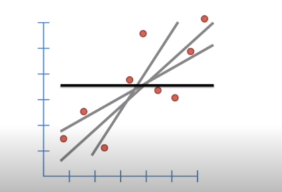
Let say the bold line (‘b’), represents the average Y value and distance between b and all the datapoints known as residual.

假設粗線('b')表示平均Y值以及b與所有稱為殘差的數據點之間的距離。

(b-Y1) is the distance between b and the first datapoint. Similarly, (b-y2) and (b-Y3) is the distance between second and third datapoints and so on.

(b-Y1)是b與第一個數據點之間的距離。 同樣，(b-y2)和(b-Y3)是第二和第三數據點之間的距離，依此類推。

Note: Some of the datapoints are less than b and some are bigger so on adding they cancel out each other, therefore we take the squares of the sum of residuals.

注意 ：有些數據點小于b，有些數據點較大，因此加起來它們會互相抵消，因此我們采用殘差總和的平方。

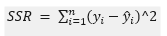
SSR = (b-Y1)2 + (b-Y2)2 + (b-Y3)2 + ………… + ……(b-Yn)2 . where, n is the number of datapoints.

SSR =(b-Y1)2+(b-Y2)2+(b-Y3)2+…………+……(b-Yn)2 。 其中，n是數據點的數量。

When for the line SSR is very less, the line is considered to be the best fit line. To find this best fit lines we need the help of equation of straight lines:

當直線的SSR很小時，該直線被認為是最合適的直線。 為了找到最佳擬合線，我們需要直線方程的幫助：

Y = mX+c

Y = mX + c

Where, m is the slope and c is the intercept through y_axis. Value of ‘m’ and ‘c’ should be optimal for SSR to be less.

其中，m是斜率，c是通過y_axis的截距。 對于SSR，“ m”和“ c”的值應最佳。

SSR = ((mX1+c)-Y1)2 + ((mX2+c)-Y2)2 + ………. + …….

SSR =((mX1 + c)-Y1)2+((mX2 + c)-Y2)2+…………。 +……。

Where Y1, Y2, ……., Yn is the observed/actual value and,

其中Y1，Y2，.......，Yn是觀測值/實際值，并且

(mX1+c), (mX2+c), ………. Are the value of line or the predicted value.

(mX1 + c)，(mX2 + c)，…………。 是線的值還是預測值。

Since we want the line that will give the smallest SSR, this method of finding the optimal value of ‘m’ and ‘c’ is called Least-Square.

由于我們要的是能夠提供最小SSR的線，因此這種找到'm'和'c'最佳值的方法稱為最小二乘 。

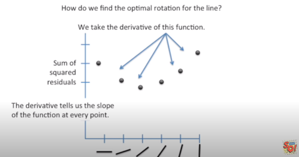
This is the plot of SSR versus Rotation of Lines. SSR goes down when we start rotating the line, and after a saturation point it starts increasing on further rotation. The line of rotation for which SSR is minimal is the best fitted line. We can use derivation for finding this line. On derivation of SSR, we get the slope of the function at every point, when at the point the slope is zero, the model select that line.

這是SSR與線旋轉的關系圖。 當我們開始旋轉線時，SSR會下降，并且在達到飽和點后，它會隨著進一步旋轉而開始增加。 SSR最小的旋轉線是最佳擬合線。 我們可以使用推導找到這條線。 在推導SSR時，我們獲得函數在每個點的斜率，當該點的斜率為零時，模型選擇該線。

R-平方 (R-Squared)

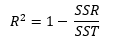
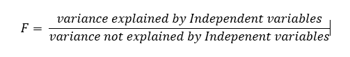
R-Squared is the goodness-of-fit measure for the linear regression model. It tells us about the percentage of variance in the dependent variable explained by Independent variables. R-Squared measure strength of relationship between our model and dependent variable on 0 to 100% scale. It explains to what extent the variance of one variable explains the variance of second variable. If R-Squared of any model id 0.5, then half of the observed variation can be explained by the model’s inputs. R-Squared ranges from 0 to 1 or 0 to 100%. Higher the R2, more the variation will be explained by the Independent variables.

R平方是線性回歸模型的擬合優度度量。 它告訴我們有關自變量解釋的因變量的方差百分比。 R平方測量模型與因變量之間的關系強度，范圍為0至100％。 它解釋了一個變量的方差在多大程度上解釋了第二個變量的方差。 如果R-Squared的任何模型id為0.5，則可以通過模型的輸入解釋觀察到的變化的一半。 R平方的范圍是0到1或0到100％。 R2越高，自變量將解釋更多的變化。

R2 = Variance explained by model / Total variance

R2=用模型解釋的方差/總方差

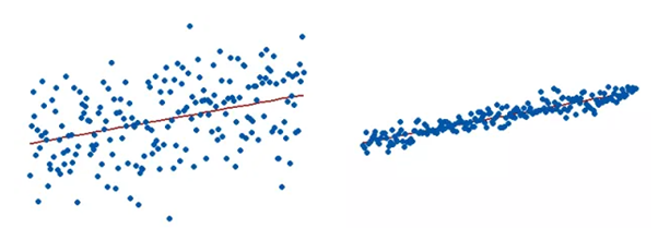
R2 for the model on left is very less than that of the right.

左側模型的R2遠小于右側模型的R2。

But it has its limitations:

但是它有其局限性：

· R2 tells us the variance in dependent variable explained by Independent ones, but it does not tell whether the model is good or bad, nor will it tell you whether the data and predictions are biased. A high R2 value doesn’t mean that model is good and low R2 value doesn’t mean model is bad. Some fields of study have an inherently greater amount of unexplained variation. In these areas R2 value is bound to be lower. E.g., study that tries to predict human behavior generally has lower R2 value.

·R2告訴我們獨立變量解釋的因變量方差，但它不告訴模型好壞，也不會告訴您數據和預測是否有偏差。 高R2值并不表示模型良好，而低R2值并不意味著模型不好。 一些研究領域固有地存在大量無法解釋的變化。 在這些區域中，R 2值必然較低。 例如，試圖預測人類行為的研究通常具有較低的R2值。

· If we keep adding the Independent variables in our model, it tends to give more R2 value, e.g., House cost prediction, number of doors and windows are the unnecessary variable that doesn’t contribute much in cost prediction but can increase the R2 value. R Squared has no relation to express the effect of a bad or least significant independent variable on the regression. Thus, even if the model consists of a less significant variable say, for example, the person’s Name for predicting the Salary, the value of R squared will increase suggesting that the model is better. Multiple Linear Regression tempt us to add more variables and in return gives higher R2 value and this cause to overfitting of model.

·如果我們繼續在模型中添加自變量，那么它往往會提供更大的R2值，例如，房屋成本預測，門窗數量是不必要的變量，雖然對成本預測的貢獻不大，但可以增加R2值。 R平方沒有關系表示不良或最不重要的自變量對回歸的影響。 因此，即使模型包含一個不太重要的變量，例如，用于預測薪水的人員姓名，R平方的值也會增加，表明該模型更好。 多元線性回歸誘使我們添加更多變量，反過來又賦予了較高的R2值，這導致模型過度擬合。

Due, to its limitation we use Adjusted R-Squared or Predicted R-Squared.

由于其局限性，我們使用調整后的R平方或預測的R平方。

Calculation of R-Squared

R平方的計算

Project all the datapoints on Y-axis and calculate the mean value. Just like SSR, sum of squares of distance between each point on Y-axis and Y-mean is known as SS(mean).

將所有數據點投影到Y軸上并計算平均值。 與SSR一樣，Y軸上每個點與Y均值之間的距離的平方和稱為SS(mean)。

Note: (I am not trying to explain it as in mathematical formula, In Wikipedia and every other place the mathematical approach is given. But this is the theoretical way and the easiest way I understood it from Stat Quest. Before following mathematical approach, we should know the concept behind this).

注意 ：(我不打算像維基百科中的數學公式那樣解釋它。 每隔一個地方都給出了數學方法。 但這是理論上的方法，也是我從Stat Quest了解它的最簡單方法。 在遵循數學方法之前，我們應該了解其背后的概念)。

SS(mean) = (Y-data on y-axis — Y-mean)2

SS(平均值)=(y軸上的Y數據-Y平均值)2

SS(var) = SS(mean) / n .. where, n is number of datapoints.

SS(var)= SS(mean)/ n ..其中，n是數據點的數量。

Sum of Square around best fit line is known as SS(fit).

最佳擬合線周圍的平方和稱為SS(擬合)。

SS(fit) = (Y-data on X-axis — point on fit line)2

SS(fit)=(X軸上的Y數據-擬合線上的點)2

SS(fit) = (Y-actual — Y-predict)2

SS(fit)=(Y實際-Y預測)2

Var(fit) = SS(fit) / n

Var(擬合)= SS(擬合)/ n

R2 = (Var(mean) — Var(fit)) / Var(mean)

R2=(Var(平均值)-Var(擬合))/ Var(平均值)

R2 = (SS(mean) — SS(fit)) / SS(mean)

R2=(SS(平均值)-SS(擬合))/ SS(平均值)

R2 = 1 — SS(fit)/SS(mean)

R2= 1-SS(擬合)/ SS(平均值)

Mathematical approach:

數學方法：

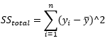
Here, SS(total) is same as SS(mean) i.e. SST (Total Sum of Squares) is the sum of the squares of the difference between the actual observed value y, and the average of the observed value (y mean) projected on y-axis.

在此，SS(total)與SS(mean)相同，即SST(總平方和)是實際觀測值y與投影到實測值y的平均值之間的差的平方之和。 y軸。

Here, SSR is same as SS(fit) i.e. SSR (Sum of Squares of Residuals) is the sum of the squares of the difference between the actual observed value, y and the predicted value (y^).

在此，SSR與SS(fit)相同，即SSR(殘差平方和)是實際觀測值y與預測值(y ^)之差的平方和。

Adjusted R-Squared:

調整后的R平方：

Adjusted R-Squared adjusts the number of Independent variables in the model. Its value increases only when new term improves the model fit more than expected by chance alone. Its value decreases when the term doesn’t improve the model fit by sufficient amount. It requires the minimum number of data points or observations to generate a valid regression model.

調整后的R平方調整模型中自變量的數量。 僅當新術語使模型的擬合度超出偶然的預期時，其價值才會增加。 當該術語不能充分改善模型擬合時，其值會減小。 它需要最少數量的數據點或觀測值才能生成有效的回歸模型。

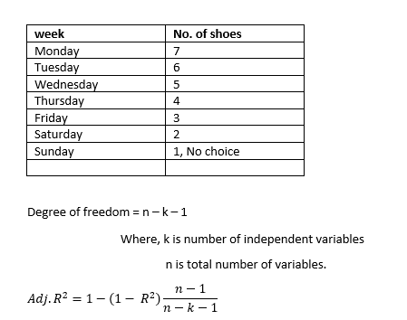
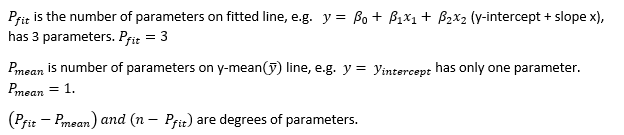
Adjusted R-Squared use Degrees of Freedom in its equation. In statistics, the degrees of freedom (DF) indicate the number of independent values that can vary in an analysis without breaking any constraints.

調整后的R平方使用自由度在其方程式中。 在統計數據中 ，自由度(DF)表示獨立值的數量，這些獨立值在分析中可以變化而不會破壞任何約束。

Suppose you have seven pair of shoes to wear each pair on each day without repeating. On Monday, you have 7 different choices of pair of shoes to wear, on Tuesday choices decreases to 6, therefore on Sunday you don’t have any choice to wear which shoes you gonna wear, you are stuck with only the last left one to wear. We have no freedom on Sunday. Therefore, degree of freedom is how much an independent variable can freely vary to analyse the parameters.

假設您每天要穿七雙鞋，而不必重復。 在星期一，您有7種不同的鞋穿選擇，在星期二，選擇的鞋數減少到6，因此在星期天，您別無選擇要穿哪雙鞋，只穿了最后一雙穿。 周日我們沒有自由。 因此，自由度是自變量可以自由變化多少以分析參數。

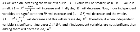
Every time you add an independent variable to a model, the R-squared increases, even if the independent variable is insignificant. It never declines. Whereas Adjusted R-squared increases only when independent variable is significant and affects dependent variable. It penalizes you for adding independent variable that do not help in predicting the dependent variable.

每次向模型添加自變量時，即使自變量無關緊要， R平方 也會增加 。 它永遠不會下降。 而僅當自變量顯著且影響因變量時， 調整后R平方才會增加。 它會因添加無助于預測因變量的自變量而受到懲罰。

for detail understanding watch Krish Naik

了解更多細節，請觀看 Krish Naik

P — Value

P —值

Suppose in a co-ordinate plane of 2-D, within the axis of x and y lies two datapoints irrespective of coordinates, i.e. anywhere in the plane. If we draw a line joining them it will be the best fit line. Again, if we change the coordinate position of those two points and again join them, then also that line will be the best fit. No matter where the datapoints lie, the line joining them will always be the best fit and the variance around them will be zero, that gives

假設在x和y軸內的2-D坐標平面中，存在兩個數據點，而與坐標無關，即平面中的任何位置。 如果我們畫一條線連接它們，那將是最合適的線。 同樣，如果我們更改這兩個點的坐標位置并再次連接它們，則該線也將是最合適的。 無論數據點位于何處，連接它們的線將始終是最佳擬合，并且它們周圍的方差將為零，從而得出

value always 100%. But that doesn’t mean those two datapoints will always be statistically significant, i.e. always give the exact prediction of target variable. To know about the statistically significant independent variables that gives good R2 value, we calculate P — value.

值始終為100％。 但這并不意味著這兩個數據點在統計上始終是有意義的，即始終給出目標變量的準確預測。 要了解具有良好R2值的統計上顯著的自變量，我們計算P —值。

Big Question — What is P — Value?

大問題-什么是P-值？

We still don’t know anything about P — Value. P — value is like Thanos and to defeat Thanos we have to deal with Infinity Stones first. P — value has its own infinity stones like alpha(α), F — score, z — score, Null Hypothesis, Hypothesis Testing, T-test, Z-test. Let’s first deal with F — score.

我們仍然對P —值一無所知。 P-價值就像Thanos并擊敗Thanos 我們必須先與Infinity Stones打交道。 P-值具有自己的無窮大石頭，例如alpha(α)，F-分數，z-分數，零假設，假設檢驗，T檢驗，Z檢驗。 首先處理F-分數。

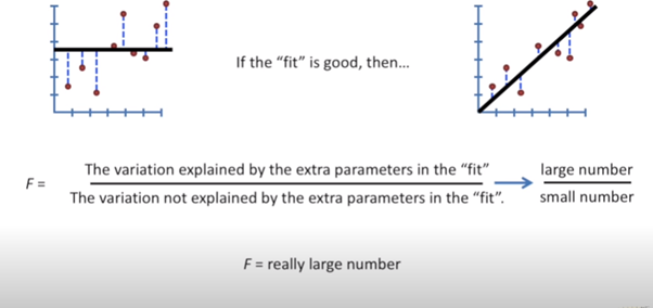
The fit line is the variance explained by the extra parameters. The distance between the fit line and the actual datapoints is known as Residuals. These Residuals are the variation not explained by the extra parameters in the fit.

擬合線是額外參數解釋的方差。 擬合線和實際數據點之間的距離稱為殘差。 這些殘差是擬合中多余參數無法解釋的變化。

For different random sets of datapoints (or samples), there will be different calculated F. let say, for thousands of samples there will be thousands of F. If we plot all the F on histogram plot, it will look something like this.

對于不同的隨機數據點集(或樣本)，將有不同的計算得出的F。可以說，對于成千上萬的樣本，將有成千上萬的F。如果我們在直方圖上繪制所有F，則看起來像這樣。

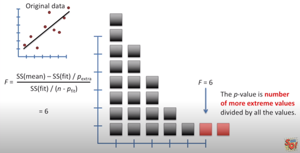
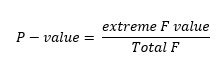
If we draw a line connecting the outer of all the F, we get like this

如果我們畫一條連接所有F外部的線，我們將得到這樣的結果

The shape of the line is been determined by the degrees of freedom

線的形狀由自由度確定

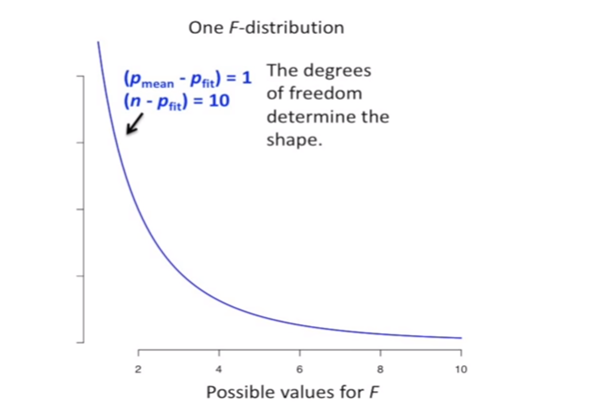
For the red line the sample size is smaller than the sample size of blue line, the blue line with more sample size is narrowing towards x-axis faster than that of red line. If the sample size is greater relative to the number of parameters in fit line then P — value will be smaller.

對于紅線，樣本大小小于藍線的樣本大小，具有更多樣本大小的藍線向x軸的收縮速度比紅線快。 如果樣本大小相對于擬合線中的參數數量更大，則P —值將更小。

For further clear understanding about P — value, we need to first understand about the Hypothesis Testing.

為了進一步清楚地了解P值，我們需要首先了解假設檢驗。

Hypothesis Testing –

假設檢驗 -

What is Hypothesis? Any guess done by us is Hypothesis. E.g.

假設是什么？ 我們所做的任何猜測都是假設。 例如

1. On Sunday, Peter always play Basketball.

1.星期天，彼得總是打籃球。

2. A new vaccine for corona will work great.

2.一種新的電暈疫苗效果很好。

3. Sachin always scores 100 on Eden.

3.薩欽(Sachin)在伊甸園(Eden)總是得分100。

4. NASA may have detected a new species.

4. NASA可能檢測到新物種。

5. I can have a dozen eggs at a time. Etc. etc.

5.我一次可以打十二個雞蛋。 等等

If we put all the above guessed sentence on a test, it is known as Hypothesis Testing.

如果我們將以上所有猜測的句子放在測試中，則稱為假設測試。

1. If tomorrow is Sunday, then Peter will be found playing Basketball.

1.如果明天是星期天，那么彼得將被發現打籃球。

2. If this is the vaccine made for corona then it will work on corona patient.

2.如果這是用于電暈的疫苗，那么它將對電暈患者有效。

3. If the match is going at Eden, then Sachin will score 100.

3.如果比賽在伊甸園進行，那么薩欽將獲得100分。

4. If there is any new species came to Earth, then it would have been detected by NASA.

4.如果有任何新物種進入地球，那么它就會被NASA探測到。

5. If I had taken part in Egg eating competition, then I could have eaten a dozen egg at a time and might have won the competition.

5.如果我參加了吃雞蛋比賽，那么我一次可以吃十幾個雞蛋，并可能贏得比賽。

6. If I regularly give water to plant, it will grow nice and strong.

6.如果我定期給植物澆水，它會長得好壯。

7. If I’ll have a good coffee in morning, then I’ll work all day without being tired. Etc. etc.

7.如果我早上可以喝杯咖啡，那么我會整天工作而不累。 等等

You make a guess (Hypothesis), put it to test (Hypothesis testing). According to the University of California, a good Hypothesis should include both “If” and “then” statement and should include independent variable and dependent variable and can be put to test.

您進行猜測(假設)，然后進行檢驗(假設測試)。 根據加利福尼亞大學的說法，一個好的假設應同時包含“ If”和“ then”陳述，并應包含自變量和因變量，并可以進行檢驗。

Null Hypothesis –

零假設 -

Null Hypothesis is the guess that we made. Any known fact can be a Null Hypothesis. Every guess we made above is Null Hypothesis. It can also be, e.g. our solar system has eight planets (excluding Pluto), Buffalo milk has more fat than that of cow, a ball will drop more quickly than a feather if been dropped freely from same height in vacuum.

零假設 是我們所做的猜測。 任何已知的事實都可以是零假設。 我們上面所做的每一個猜測都是零假設。 也可能是這樣的，例如我們的太陽系有八個行星(不包括冥王星)，水牛乳的脂肪比牛的脂肪多，如果在真空中從相同高度自由掉落，則球掉落的速度將比羽毛快。

Now here’s a catch. We can accept the Null Hypothesis or can reject the Null Hypothesis. We perform test on Null Hypothesis based on same observation or data, if the Hypothesis is true then we accept it or else we reject it.

現在有一個陷阱。 我們可以接受零假設，也可以拒絕零假設。 我們基于相同的觀察或數據對空假設進行檢驗，如果假設為真，則我們接受該假設，否則我們拒絕該假設。

Big Question? How this test is done?

大問題？ 該測試如何完成？

We evaluate two mutual statement on a Population (millions of data containing Independent and dependent variables) data using sample data (randomly chosen small quantity of data from a big data). For testing any hypothesis, we have to follow few steps:

我們使用樣本數據(從大數據中隨機選擇的少量數據)評估總體 ( 人口數據(包含自變量和因變量的數百萬個數據))上的兩個相互陳述。 為了檢驗任何假設，我們必須遵循幾個步驟：

1. Make an assumption.

1.做一個假設。

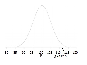
For e.g. let say A principal at a certain school claims that the students in his school are above average intelligence. A random sample of thirty students IQ scores have a mean score of 112. Is there sufficient evidence to support the principal’s claim? The mean population IQ is 100 with a standard deviation of 15.

例如，假設某所學校的一位校長聲稱他所在學校的學生的智力高于平均水平。 隨機抽取 30名學生的智商得分， 平均得分為112。是否有足夠的證據支持校長的主張？ 總體智商平均為100， 標準差為15。

Here the Null Hypothesis is the accepted fact that the average IQ is 100. i.e.

在這里，零假設是公認的事實，即平均智商為100。即

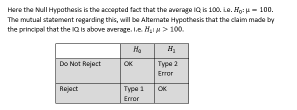
Let say that after testing our Null Hypothesis is true, i.e. the claim made by principal that average IQ of students is above 100 is wrong. We chosen different sets of 30 students and took their IQ and averaged it and found in most cases that the average IQ is not more than 100. Therefore, our Null Hypothesis is true and we reject Alternate Hypothesis. But let say that due to lack of evidence we can’t able to find out the result or somehow mistakenly (two or three students are exceptionally brilliant with much more IQ) we calculated that average IQ is above 100 but the actual correct result is average IQ is 100 and we reject Null Hypothesis, this is Type 1 error.

可以說，在檢驗了我們的零假設之后，就是正確的，也就是說，校長聲稱學生的平均智商高于100是錯誤的。 我們選擇了30個學生的不同集合，并對其智商進行平均，發現在大多數情況下，平均智商不超過100。因此，我們的零假設是真實的，而我們拒絕替代假設。 但是可以說，由于缺乏證據，我們無法找到結果或以某種方式錯誤地發現(兩到三名學生非常聰明，智商更高)，我們計算出平均智商高于100，但實際正確結果是平均IQ為100，我們拒絕空假設，這是1類錯誤。

Again, let say that the Null Hypothesis is true, average IQ of students is not more than 100. But due to presence of those exceptionally brilliant students we got the average IQ above 100, so we do not reject Alternate Hypothesis. That is type 2 error.

再次，讓我們假設“零假設”是正確的，學生的平均智商不超過100。但是，由于這些出色的學生的存在，我們使平均智商高于100，因此我們不會拒絕“替代假設”。 那是類型2錯誤。

It’s confusing though. Okay let’s take another example.

不過這很令人困惑。 好吧，讓我們再舉一個例子。

Suppose a person is somehow convicted but he is innocent, he just accidentally found present near a dead body and got convicted. Here Null Hypothesis, is person is innocent. Alternate Hypothesis can be that person is guilty but due to lack of evidence, person got charged and punished by law. So, it is Type 1 error. But what if person is actually guilty. He claimed that he is innocent, Alternate hypothesis suggested he is guilty but due to lack of evidence, he got bailed and charged free. This is type 2 error (not rejecting Alternate Hypothesis).

假設某人被定罪，但他是無辜的，他只是偶然發現尸體附近存在并被定罪。 在這里零假設，就是人無辜。 替代假設可能是某人有罪，但由于缺乏證據，該人被起訴并受到法律制裁。 因此，這是Type 1錯誤。 但是如果人確實有罪怎么辦。 他聲稱自己是無辜的，另一種假設表明他有罪，但由于缺乏證據，他獲得了保釋并被釋放。 這是2類錯誤(不拒絕替代假設)。

1. Choose the alpha(α), α is the significance level which is probability of making wrong decision when Null Hypothesis is true, i.e. probability of making type 1 error. Generally, we choose α = 0.05, it’s okay if for less than 5 % of cases Null Hypothesis is proven wrong, we still consider it. But if Null hypothesis is wrong more than in 5% case then we reject it and accept Alternate Hypothesis. For important decision, like in medical cases or share market we do not take α > 0.03, it could be risk even if we avoid a minute error in these cases.
   選擇alpha(α)，α是顯著性水平，當無效假設為真時，它是做出錯誤決策的概率，即發生類型1錯誤的概率。 通常，我們選擇α= 0.05，如果在不到5％的情況下，零假設被證明是錯誤的，我們仍然會考慮，那就可以了。 但是，如果空假設的錯誤率超過5％，則我們將其拒絕并接受替代假說。 對于重要決策，例如在醫療案例或股票市場中，我們不使α> 0.03，即使在這些案例中避免了微小的誤差，也可能存在風險。
2. 1. Perform the test.
   1.執行測試。

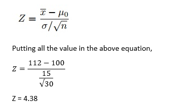
Z— test

Z—檢驗

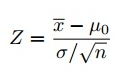
Here, X(bar) is the sample mean, i.e. Average IQ of randomly chosen 30 students which is 112.

這里的X(bar)是樣本平均值，即隨機選擇的30名學生的平均智商為112。

(Mu-0) is the population mean, i.e. Average IQ of all students that is 100.

(Mu-0)是人口平均值，即所有學生的平均智商為100。

(sigma) is the standard deviation, i.e. how much data is varying from the population mean?

(sigma)是標準偏差，即，與總體平均值相比有多少數據不同？

n is the sample size that is 30.

n是30的樣本量。

Let’s discuss about the Normal distribution and Z-score before performing the test.

在執行測試之前，讓我們討論正態分布和Z分數。

Normal Distribution

正態分布

Properties:

特性：

· Bell shaped curve

·鐘形曲線

· No skewness

·無偏斜

· Symmetrical

·對稱

· In normal distribution,

·在正態分布中，

Mean = median = mode

平均值=中位數=模式

Area Under Curve is 100% or 1

曲線下面積為100％或1

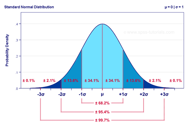
Mean = 0 and standard deviation, σ = 1

均值= 0和標準偏差σ= 1

Z — score

Z-得分

Z — score tells us that how much a data, a score, a sample is been deviated from the mean of normal distribution. By the help of Z — score we can convert any score or sample distribution with mean and standard deviation other than that of a normal distribution, (i.e. when the data is skewed) to the mean and deviation of normal distribution of mean equal to zero and deviation equal to one.

Z-得分 告訴我們，數據，得分，樣本有多少偏離了正態分布的均值。 借助Z-評分，我們可以將除正態分布外的均值和標準差(即，當數據偏斜時)的任何得分或樣本分布轉換為均值和均值的正態分布與均值的偏差，均值等于零，偏差等于一。

From Z — score table, an area of α = 0.05 is equal to 1.645 of Z — score, which is smaller than Z value we get. So we will reject the Null Hypothesis in this case.

從Z_分數表中 ， α= 0.05的面積等于Z_分數的1.645，小于我們得到的Z值。 因此，在這種情況下，我們將拒絕零假設。

Now, we got the Z — score, we can calculate P — value, by the help of Normal Distribution Table:

現在，我們得到了在Z -得分，我們可以計算出P -值 ，通過幫助正態分布表：

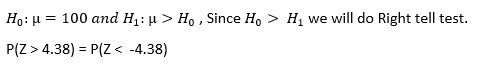
By looking at Normal Distribution table we get that Z — value for the value less than — 3 is 0.001. If the P — value < 0.05, we reject the Null Hypothesis.

通過查看正態分布表，我們得出Z值小于-3的值為0.001。 如果P值<0.05，則我們拒絕零假設。

Big.. Big Confusion –

大..大混亂–

We often tend to confuse between probability and P — value. But there is a big difference between them. Let’s take an example.

我們常常傾向于混淆概率和P值。 但是它們之間有很大的區別。 讓我們舉個例子。

By flipping a coin, we can get the chance of coming of head is 50%. If we flip another coin, again the chance of getting a head is 50%.

通過擲硬幣，我們可以獲得正面的機會是50％。 如果我們擲另一枚硬幣，再次獲得正面的機會是50％。

Now, what’s the probability of getting two head in a row and what’s the P — value of getting two head in a row?

現在，連續獲得兩個頭的概率是多少？連續獲得兩個頭的P值是多少？

On flipping of two coins simultaneously,

同時翻轉兩枚硬幣時，

Total outcome = HH, HT, TH, TT = 4

總結果= HH，HT，TH，TT = 4

Favorable outcome = HH = 1

有利的結果= HH = 1

P(HH) = ? = 0.25, and P(TT) = ? = 0.25

P(HH)=?= 0.25，P(TT)=?= 0.25

P(one H or one T) =(HT,TH)/(HH,HT,TH,TT)=2/4=0.5

P(一個H或一個T)=(HT，TH)/(HH，HT，TH，TT)= 2/4 = 0.5

P — value is the probability that the random chance generated the data, or something else that is equal or rarer.

P —值是隨機機會生成數據的概率，或者等于或稀少的其他概率。

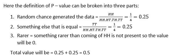
Therefore, probability of getting two heads in a row is 0.25 and P — value for getting two heads in a row is 0.5.

因此，連續獲得兩個頭的概率為0.25，連續獲得兩個頭的P_值為0.5。

All the graphical plots are taken from Stat Quest. for this article I have followed Stat Quest and Krish Naik.

所有圖形圖均取自Stat Quest。 對于本文，我關注了Stat Quest和Krish Naik 。

If something is missing here or explained wronged, then please comment and guide me through it.

如果此處缺少或解釋有誤，請發表評論并指導我。