Customizing a graph to transform it into a beautiful figure in R isn’t alchemy. Nonetheless, it took me a lot of time (and frustration) to figure out how to make these plots informative and publication-quality. Rather than hoarding this information like a dragon presiding over its treasure, I want to share the code I use to plot data, explaining what each piece of it does.

自定義圖形以將其轉換為R中的漂亮圖形并不是煉金術。 盡管如此，我還是花了很多時間(和沮喪)來弄清楚如何使這些情節具有信息性和出版質量。 我要分享的是我用來繪制數據的代碼，而不是像巨龍一樣掌控著它的寶藏，而是解釋了每個信息的作用。

First thing’s first, let’s load our packages and generate a dummy dataset, with one independent variable and one continuous dependent variable. Before the code snippet, I’ll discuss the functions and arguments we will use. We also set an order for our categorical variables beforehand.

首先，讓我們加載包并生成一個虛擬數據集，其中包含一個自變量和一個連續因變量。 在代碼片段之前，我將討論我們將使用的函數和參數。 我們還預先為分類變量設置了順序。

虛擬數據集：函數和參數 (Dummy Dataset: Functions and arguments)

• runif generates 100 numbers between 0 and 1

  runif生成100個介于0和1之間的數字

• sample randomly selects the number 1 or 2, 100 times

  樣本隨機選擇數字1或2，進行100次

• factor sets a preferred order for our grouping variables

  因子為分組變量設置了首選順序

### Load packages
install.packages('ggplot2')
install.packages('RColorBrewer')
install.packages('ggpubr')
library(ggplot2)
library(RColorBrewer)
library(ggpubr)#Create dummy dataset
ndf <- data.frame(
  value     = rep(runif(100)), 
  factor1   = as.char(rep(sample(1:2, replace = TRUE, 100))
)
ndf$factor1 = factor(ndf$factor1, levels = c('1', '2'))

箱形圖：函數和參數 (Box Plot: Functions and Arguments)

• ggplot allows us to specify the independent and dependent variables, as well as the dataset to use for the graph

  ggplot允許我們指定自變量和因變量，以及用于圖的數據集

• stat_boxplot lets us specify the type of whiskers to add onto the plot

  stat_boxplot讓我們指定要添加到繪圖中的晶須類型

• geom_boxplot specifies the independent and dependent variables for the boxes in the plot

  geom_boxplot為圖中的框指定自變量和因變量

The first basic attempt isn’t very informative or visually appealing. We focus first on just plotting the first independent variable, factor1. I also don’t like the default grey theme within ggplot.

最初的基本嘗試不是很有啟發性或視覺吸引力。 我們首先專注于繪制第一個自變量factor1。 我也不喜歡ggplot中的默認灰色主題。

plot_data <- ggplot(ndf, aes(y = value, x = factor1)) +
  stat_boxplot( aes(y = value, x = factor1 ), 
                geom='errorbar', width=0.5) +
  geom_boxplot(aes(y = value, x =  factor1))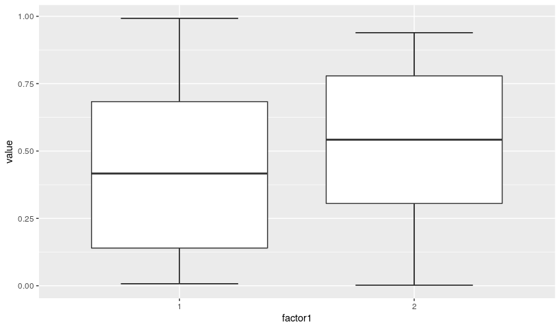

帶點的箱形圖：函數和參數 (Box Plot with Dots: Functions and Arguments)

• theme_bw() sets a black-and-white theme for the plot, getting rid of the pesky grey background

  theme_bw()為情節設置了黑白主題，擺脫了討厭的灰色背景

• geom_dotplot: binaxis specifies which variable will be displayed with the dots. The other arguments specify the appearance of the dots, while binwidth specifies how many dots we want in the same row on our plot. If you want to make the dots see-through, use the alpha argument which lets you specify the opacity of the dots from 0 to 1.

  geom_dotplot： binaxis指定將與點一起顯示的變量。 其他參數指定點的外觀，而binwidth指定在繪圖的同一行中需要多少個點。 如果要使點透明，請使用alpha參數，該參數可以指定點的不透明度從0到1。

Now our plot is more informative but it still needs improvement. We want to modify some of the colors, axes and labels.

現在我們的情節提供了更多信息，但仍需要改進。 我們要修改一些顏色，軸和標簽。

plot_data <- ggplot(ndf, aes(y = value, x = factor1)) +
    stat_boxplot( aes(y = value, x = factor1 ), 
                  geom='errorbar', width = 0.5) +
    geom_boxplot(aes(y = value, x =  factor1)) +
      theme_bw() +
      geom_dotplot(binaxis='y', 
                   stackdir = "center", 
                   binwidth = 1/20,
                   dotsize = 1, 
                   aes(fill = factor1))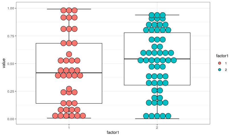

出汗的小事情 (Sweating the Little Things)

• scale_fill_manual lets us set specific colors for specific values of our independent variables

  scale_fill_manual讓我們為自變量的特定值設置特定的顏色

• xlab and ylab allow us to label the x and y axis respectively. If you put the escape character following the newline symbol into the title (\n) it continues the rest of the label on the next line!

  xlab和ylab允許我們分別標記x和y軸。 如果將換行符后面的轉義字符放在標題(\ n)中，它將在下一行繼續其余標簽！

• ggtitle names your plot

  ggtitle為您的情節命名

• theme is a very customizable part of the script. It let’s us customize just about anything we want with its arguments. Since I don’t like the default grids placed in ggplots, I attribute element_blank to a few panel arguments to get rid of the border around the plot. I make the axis colored black rather than grey. I also specify how much blank space I want around the graph with plot_margin. Since this plot is simple, we get rid of the legend for this example. With the various axis_text arguments I set the size, font face, color and positioning of axis text and labels.

  主題是腳本中非常可定制的部分。 它使我們可以自定義幾乎所有我們想要的參數。 由于我不喜歡放置在ggplots中的默認網格，因此我將element_blank賦予一些面板參數以擺脫繪圖周圍的邊界。 我將軸設為黑色而不是灰色。 我還使用plot_margin指定想要在圖形周圍留多少空白。 由于該圖很簡單，因此在此示例中，我們擺脫了圖例。 通過各種axis_text參數，我設置了軸文本和標簽的大小，字體，顏色和位置。

• scale_y_continuous sets the y axis increases from 0 to 1 in 0.2 intervals. By expanding the limit of the plot beyond 1, it gives the title more breathing room. If I needed to use a y-axis with discrete variable names, I could use a different argument — scale_y_discrete.

  scale_y_continuous設置y軸以0.2的間隔從0增加到1。 通過將圖的限制擴展到超過1，可以為標題提供更多的喘息空間。 如果我需要使用帶有離散變量名稱的y軸，則可以使用其他參數-scale_y_discrete。

• scale_x_discrete lets me relabel the two independent variables. This lets you quickly rename codified data. I’ve relabeled the independent variables as Danny DeVito and Nicolas Cage. Let’s posit that we are looking at how well Nic Cage and Danny DeVito performed at the box office using scores scaled between 0 and 1.

  scale_x_discrete讓我重新標記兩個自變量。 這使您可以快速重命名編碼的數據。 我將自變量重新標記為Danny DeVito和Nicolas Cage。 假設我們正在研究Nic Cage和Danny DeVito在0和1之間的得分在票房上的表現。

• stat_compare_means lets you do statistical tests. This one’s here for you to explore! Just type stat_compare_means( and press tab to explore the different options available to you. Otherwise you can type ?stat_compare_means to get the help manual for this function!

  stat_compare_means使您可以進行統計檢驗。 這個在這里供您探索！ 只需鍵入stat_compare_means(并按Tab鍵即可探索可用的其他選項。否則，您可以鍵入？stat_compare_means以獲得此功能的幫助手冊！

If you’re wondering about the hjust and vjust within different elements of the code, it simply allows us to change position of text elements. I added some flare by changing the boxplot line coloring as well as the fill of our dots. If you’re building a busy plot, it’s also important to check for accessibility. You can find colorblind friendly palette with this tool: https://colorbrewer2.org/.

如果您想知道代碼中不同元素之間的平衡，它只是允許我們更改文本元素的位置。 我通過更改箱形圖線的顏色以及點的填充來增加了耀斑。 如果您要建立繁忙的地塊，檢查可訪問性也很重要。 您可以使用此工具找到對色盲友好的調色板： https : //colorbrewer2.org/ 。

For convenience, I’ve bolded any changes in the code for the plot to make it easier to follow.

為了方便起見，我將圖中代碼的所有更改加粗了，以使其易于理解。

plot_data <- ggplot(ndf, 
                    aes(y = value, x = factor1, color = factor1))+
                    scale_color_manual(values = 
                                       c('1' = 'blue', 
                                         '2' = 'firebrick4')) +
      stat_boxplot( aes(y = value, x = factor1 ), 
                    geom='errorbar', width = 0.5) +
      geom_boxplot(aes(y = value, x =  factor1), shape = 2)+
                         theme_bw() +
        geom_dotplot(binaxis='y', 
                     stackdir = "center", 
                     binwidth = 1/20,
                     dotsize = 1,
                     aes(fill = factor1)) + 
  scale_fill_manual(values = c('1' = '#0571b0', '2' = '#ca0020')) +
  xlab("Independent\nVariable") + ylab("Dependent\nVariable") +
  ggtitle("Box-Dot Plot") +
  theme(  panel.grid.major = element_blank(),
          panel.grid.minor = element_blank(), 
          axis.line = element_line(colour = "black"), 
          panel.border = element_blank(), 
          plot.margin=unit(c(0.5,0.5, 0.5,0.5),"cm"), 
          legend.position="none", 
          axis.title.x= element_text(size=14, color = 'black', vjust = 0.5),
          axis.title.y= element_text(size=14, color = 'black', vjust = 0.5),
          axis.text.x = element_text(size=12, color = 'black'),
          axis.text.y = element_text(size=14, color = 'black'),
          plot.title  = element_text(hjust = 0.5, size=16, face = 'bold', vjust = 0.5)) +
    scale_y_continuous(expand = c(0,0), breaks = seq(0,1,0.2),
                   limits = c(0,1.1)) +
    scale_x_discrete(labels = c('Nicholas Cage', 'Danny DeVito'))    stat_compare_means(method = 't.test', hide.ns = FALSE, size = 4,   vjust = 2)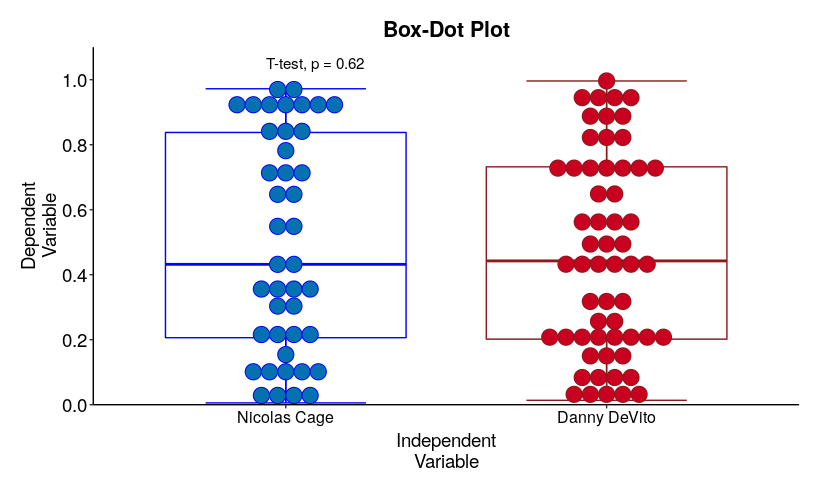

In a very short span of time, we’ve gone from a simple boxplot to a more visually appealing, accessible plot that gives us more information about the individual datapoints. You can save the code and modify it as you wish whenever you need to plot data. This makes the customization process so much easier! No more (okay maybe a lot less) computer defenestrations!

在很短的時間內，我們已經從簡單的箱形圖變成了更具視覺吸引力的可訪問圖，它為我們提供了有關各個數據點的更多信息。 您可以在需要繪制數據時保存并根據需要修改代碼。 這使定制過程變得非常容易！ 沒有更多(好的，也許更少)計算機故障！

If you’re looking to download the code, find it here: https://github.com/simon-sp/R_ggplot_basic_dotplot. I’ve left plenty of comments within the code to help you out in case you get stuck! Remember that placing a question mark before a function brings up an instruction guide for you in RStudio!

如果您要下載代碼，請在這里找到它： https : //github.com/simon-sp/R_ggplot_basic_dotplot 。 我在代碼中留下了很多注釋，以幫助您避免被卡住！ 請記住，在功能之前加一個問號會在RStudio中為您提供指導指南！