忙了一陣子,回來繼續更新
3.3 代價函數公式
In order to implement linear regression. The first key step is first to define something called a cost function. This is something we’ll build in this video, and the cost function will tell us how well the model is doing so that we can try to get it to do better. Let’s look at what this means.
為了實現線性回歸,第一個關鍵步驟是先定義一個叫作代價函數的東西。在此視頻中,我們將構建這個代價函數,代價函數將告訴我們模型的表現如何,以便我們可以嘗試使模型變得更好。讓我們看看代價函數是什么意思。
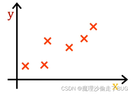
Recall that you have a training set that contains input features x and output targets y. The model you’re going to use to fit this training set is this linear function f_w, b of x equals to w times x plus b. To introduce a little bit more terminology the w and b are called the parameters of the model.
回想一下,你有一個包含輸入特征 x 和輸出目標 y 的訓練集。你要使用的模型是用來將這個訓練集的數據擬合為一個線性函數 f w , b ( x ) = w x + b f_{w,b}(x)=wx+b fw,b?(x)=wx+b。為了描述的更專業一些,我們將 w w w和 b b b 稱為模型的參數。
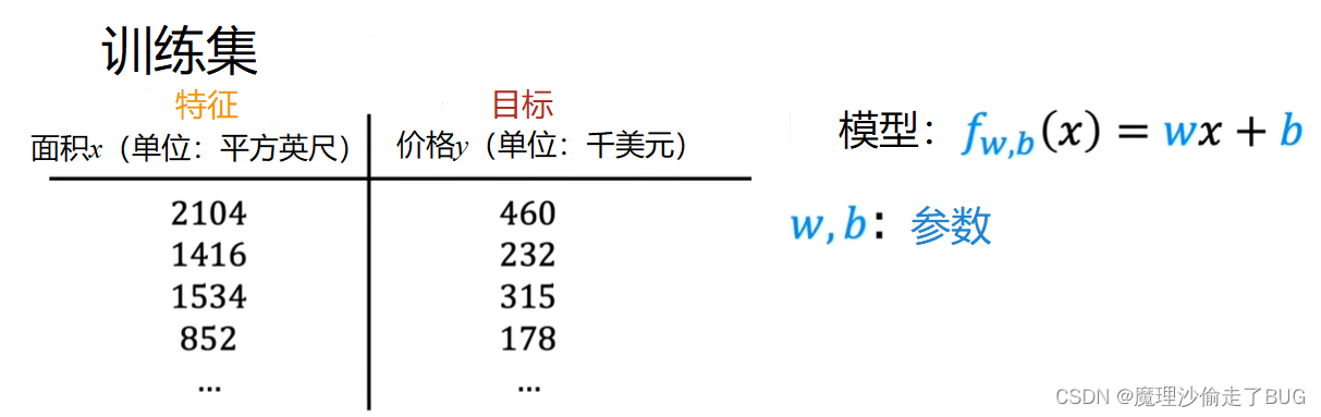
In machine learning parameters of the model are the variables you can adjust during training in order to improve the model. Sometimes you also hear the parameters w and b referred to as coefficients or as weights. Now let’s take a look at what these parameters w and b do.
在機器學習中,模型的參數是可以在訓練過程中進行調整以改善模型性能的變量。有時你也會聽到參數 w w w 和 b b b 被稱為系數或權重。現在讓我們來看看這些參數 w w w 和 b b b 的作用。
Depending on the values you’ve chosen for w and b you get a different function f of x, which generates a different line on the graph. Remember that we can write f of x as a shorthand for f_w, b of x. We’re going to take a look at some plots of f of x on a chart.
根據所選擇的 w w w 和 b b b 的值,你會得到一個不同的函數 f ( x ) f(x) f(x),這將在圖表上生成一條不同的線。記住,我們可以用 f ( x ) f(x) f(x)來簡寫 f w , b ( x ) f_{w, b}(x) fw,b?(x)。接下來,我們將看一些 f ( x ) f(x) f(x) 在圖表上的繪圖。
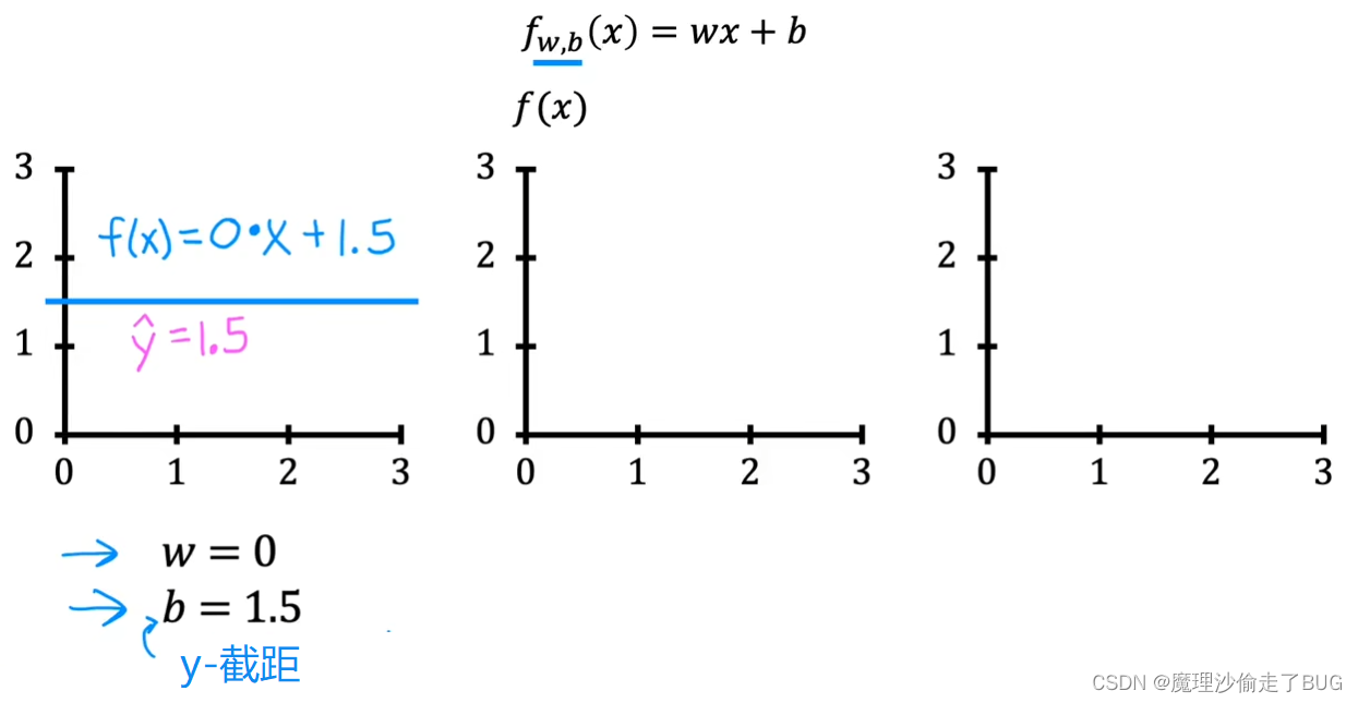
Maybe you’re already familiar with drawing lines on charts, but even if this is a review for you, I hope this will help you build intuition on how w and b the parameters determine f. When w is equal to 0 and b is equal to 1.5, then f looks like this horizontal line. In this case, the function f of x is 0 times x plus 1.5 so f is always a constant value. It always predicts 1.5 for the estimated value of y. Y hat is always equal to b and here b is also called the y intercept because that’s where it crosses the vertical axis or the y axis on this graph.
也許你已經熟悉在圖表上繪制線條,但即使這對你來說是復習,我希望這能幫助你建立如何用參數 w w w 和 b b b 確定函數 f f f的直覺。當 w = 0 w=0 w=0, b = 1.5 b=1.5 b=1.5時,函數 f f f 就像是一條水平線。在這種情況下,函數 f ( x ) = 0 × x + 1.5 f(x)=0\times x+1.5 f(x)=0×x+1.5 ,因此 f f f 始終是一個常數值。它總是對估計的 y y y 值預測為 1.5。 y ^ = b \hat y=b y^?=b,而在這里 b b b也被稱為 y y y截距(y intercept),因為它是函數在圖表上穿過垂直軸或y軸的位置。
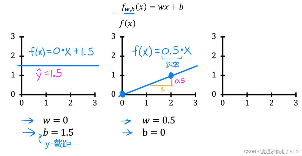
As a second example, if w is 0.5 and b is equal 0, then f of x is 0.5 times x. When x is 0, the prediction is also 0, and when x is 2, then the prediction is 0.5 times 2, which is 1. You get a line that looks like this and notice that the slope is 0.5 divided by 1. The value of w gives you the slope of the line, which is 0.5.
作為第二個示例,如果 w = 0.5 w=0.5 w=0.5, b = 0 b=0 b=0,那么 f ( x ) = 0.5 x f(x)=0.5x f(x)=0.5x. 當 x = 0 x=0 x=0時,預測值也為0,當 x = 2 x=2 x=2時,預測值就是 0.5 × 2 = 1 0.5\times 2=1 0.5×2=1. 你會得到一條看起來像這樣的線,并且注意到斜率是 0.5 1 \frac{0.5}{1} 10.5?。而 w w w的值給出了線條的斜率,也就是0.5。
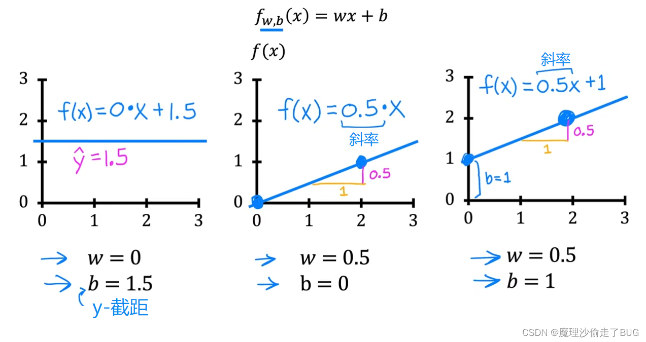
Finally, if w equals 0.5 and b equals 1, then f of x is 0.5 times x plus 1 and when x is 0, then f of x equals b, which is 1 so the line intersects the vertical axis at b, the y intercept. Also when x is 2, then f of x is 2, so the line looks like this. Again, this slope is 0.5 divided by 1 so the value of w gives you the slope which is 0.5.
最后,如果 w = 0.5 w=0.5 w=0.5, b = 1 b=1 b=1,那么 f ( x ) = 0.5 x + 1 f(x)=0.5x+1 f(x)=0.5x+1. 當 x = 0 x=0 x=0時, f ( x ) = b f(x)=b f(x)=b,也就是1,因此線條與垂直軸在b處相交,即y截距。此外,當 x = 2 x=2 x=2時, f ( x ) = 2 f(x)=2 f(x)=2,因此線條呈現如下形狀。同樣,這個斜率是 0.5 1 \frac{0.5}{1} 10.5?,因此 w w w的值給出了斜率,即0.5。
Recall that you have a training set like the one shown here. With linear regression, what you want to do is to choose values for the parameters w and b so that the straight line you get from the function f somehow fits the data well. Like maybe this line shown here.
回想一下,你有一個類似于這里展示的訓練集。
在線性回歸中,你希望選擇參數 w w w和 b b b的值,使得由函數f生成的直線與數據相擬合得較好,就像這里展示的這條線一樣。
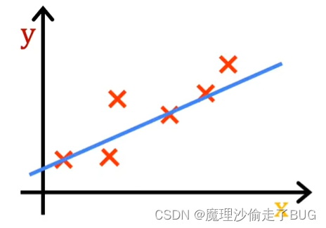
When I see that the line fits the data visually, you can think of this to mean that the line defined by f is roughly passing through or somewhere close to the training examples as compared to other possible lines that are not as close to these points. Just to remind you of some notation, a training example like this point here is defined by x superscript i, y superscript i where y is the target.
當我看到直線在視覺上與數據擬合時,你可以這樣理解,相對于其他可能不太接近這些點的直線,由函數 f f f所定義的直線大致通過或接近于訓練樣本組成的集合。再次提醒一下符號的表示,像這個點一樣的訓練樣本被定義為 x ( i ) x^{(i)} x(i)、 y ( i ) y^{(i)} y(i),其中 y y y是目標值。
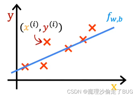
For a given input x^i, the function f also makes a predictive value for y and a value that it predicts to y is y hat i shown here. For our choice of a model f of x^i is w times x^i plus b. Stated differently, the prediction y hat i is f of wb of x^i where for the model we’re using f of x^i is equal to wx^i plus b.
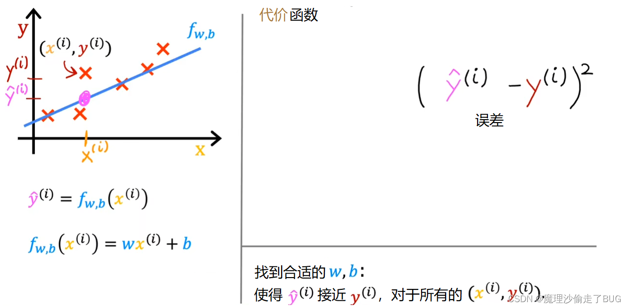
對于給定的輸入 x ( i ) x^{(i)} x(i),函數 f f f還會對 y y y有一個預測的值,表示為 y ^ ( i ) \hat y^{(i)} y^?(i)。我們選擇的模型 f f f對于輸入 x ( i ) x^{(i)} x(i)的表達式是 f ( x ) = w x ( i ) + b f(x)=wx^{(i)}+b f(x)=wx(i)+b. 換句話說,預測值 y ^ ( i ) \hat y^{(i)} y^?(i)可以表示為 y ^ ( i ) = f w , b ( x ( i ) ) \hat y^{(i)}=f_{w,b}(x^{(i)}) y^?(i)=fw,b?(x(i)),其中對于我們使用的模型, f w , b ( x ( i ) ) = w x ( i ) + b f_{w,b}(x^{(i)})=wx^{(i)}+b fw,b?(x(i))=wx(i)+b.

Now the question is how do you find values for w and b so that the prediction y hat i is close to the true target y^i for many or maybe all training examples x^i, y^i. To answer that question, let’s first take a look at how to measure how well a line fits the training data. To do that, we’re going to construct a cost function.
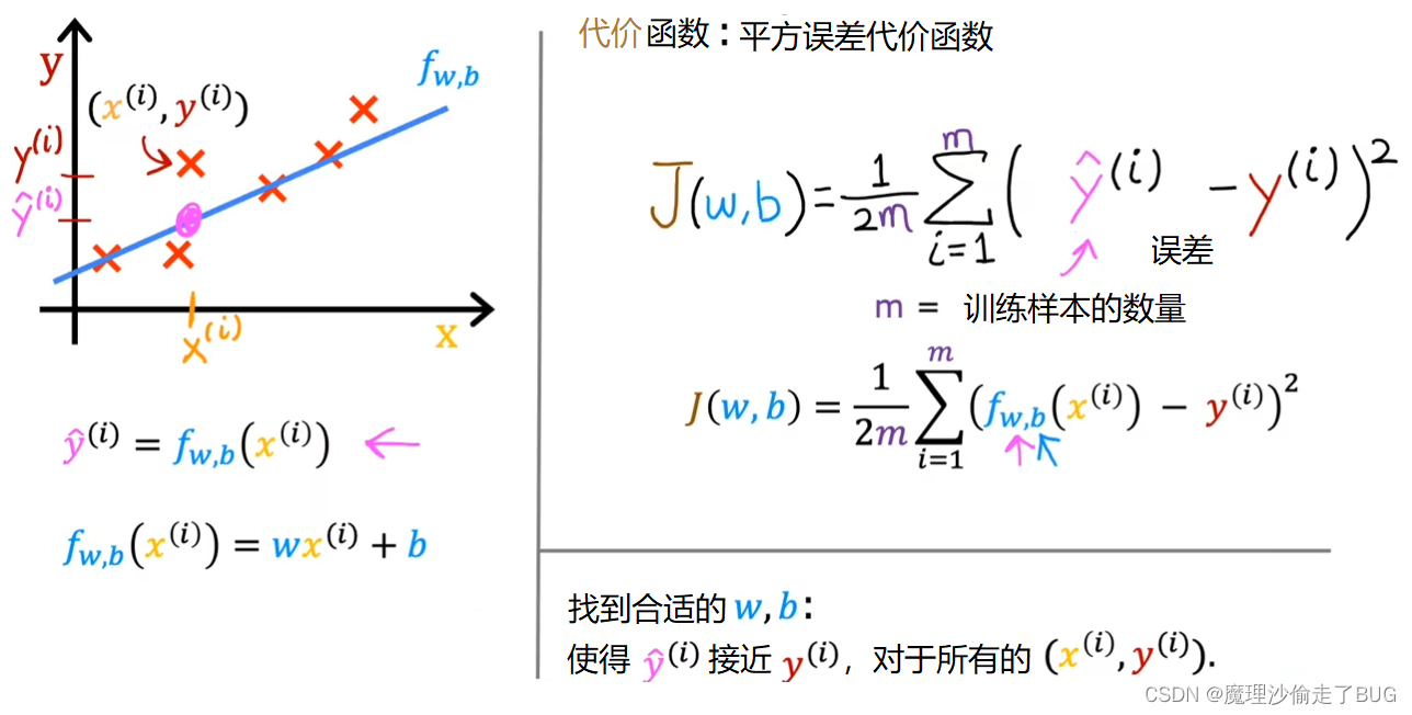
現在的問題是如何找到參數 w w w和 b b b的值,使得對于許多或者所有的訓練樣本 x ( i ) x^{(i)} x(i)、 y ( i ) y^{(i)} y(i),預測值 y ^ ( i ) \hat y^{(i)} y^?(i)與真實目標值 y ( i ) y^{(i)} y(i)接近。為了回答這個問題,讓我們首先看一下如何衡量一條直線對訓練數據的擬合程度。為此,我們將構建一個代價函數(cost function)。
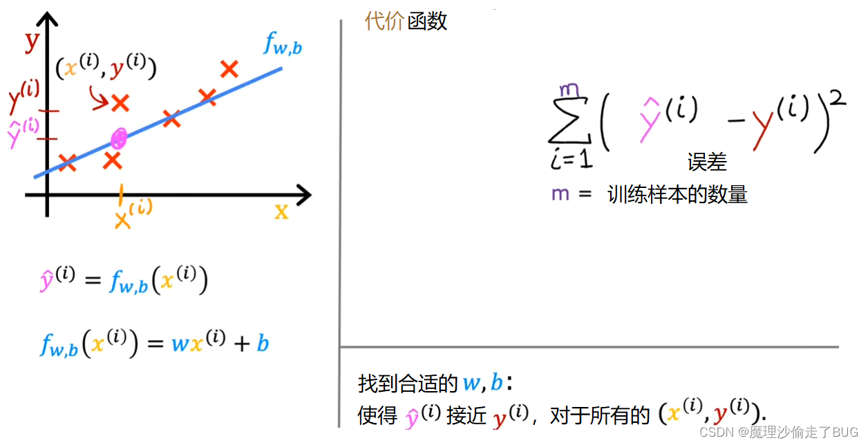
The cost function takes the prediction y hat and compares it to the target y by taking y hat minus y. This difference is called the error, we’re measuring how far off to prediction is from the target. Next, let’s computes the square of this error. Also, we’re going to want to compute this term for different training examples i in the training set. When measuring the error, for example i, we’ll compute this squared error term.
代價函數將預測值 y ^ \hat y y^?與真實的目標值 y y y進行比較,通過計算 y ^ ? y \hat y-y y^??y得到一個差值。這個差值被稱為誤差(error),我們測量了預測值與目標值之間的偏差大小。接下來,我們會計算這個誤差的平方。同時,對于訓練集中的第 i i i個樣本,我們需要計算每個樣本的預測值和真實值之間的誤差。當我們計算誤差時,比如,對于第 i i i個訓練樣本,我們將計算這個平方誤差項 y ^ ( i ) ? y ( i ) \hat y^{(i)}-y^{(i)} y^?(i)?y(i).
Finally, we want to measure the error across the entire training set. In particular, let’s sum up the squared errors like this. We’ll sum from i equals 1,2, 3 all the way up to m and remember that m is the number of training examples, which is 47 for this dataset.
最后,我們希望衡量整個訓練集上的誤差。具體而言,我們將按照如下方式將這些平方誤差求和,即 ∑ i = 1 m ( y ^ ( i ) ? y ( i ) ) 2 \displaystyle \sum_{i=1}^{m}(\hat y^{(i)}-y^{(i)})^{2} i=1∑m?(y^?(i)?y(i))2,需要記住 m m m是訓練樣本的數量,對于這個數據集來說 m = 47 m=47 m=47。
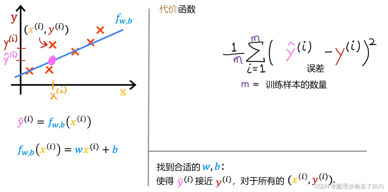
Notice that if we have more training examples m is larger and your cost function will calculate a bigger number. This is summing over more examples. To build a cost function that doesn’t automatically get bigger as the training set size gets larger by convention, we will compute the average squared error instead of the total squared error and we do that by dividing by m like this.
請注意,如果我們有更多的訓練樣本,即m更大,那么你的代價函數會計算一個更大的數值。這是因為我們對更多的樣本進行求和操作。為了構建一個無論訓練集大小如何都不會自動增大的代價函數,我們通常計算平均平方誤差而不是總平方誤差,這可以通過除以 m m m來實現,如下所示。
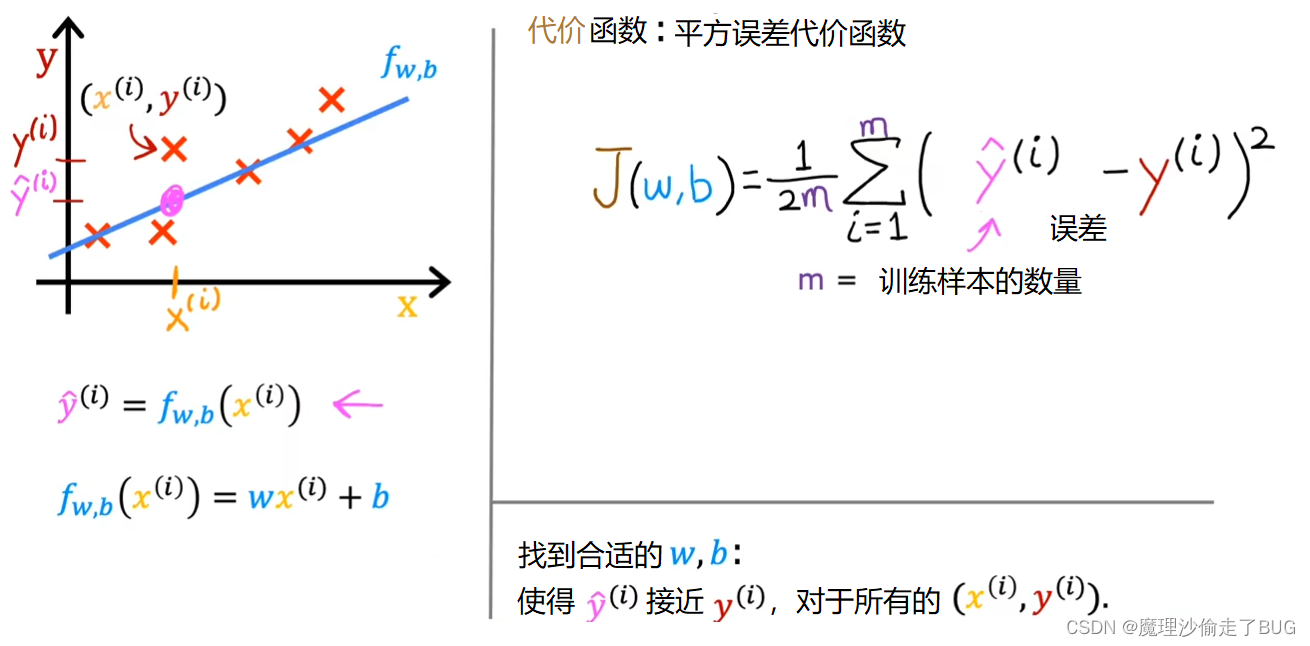
We’re nearly there. Just one last thing. By convention, the cost function that machine learning people use actually divides by 2 times m. The extra division by 2 is just meant to make some of our later calculations look neater, but the cost function still works whether you include this division by 2 or not. This expression right here is the cost function and we’re going to write J of wb to refer to the cost function. This is also called the squared error cost function, and it’s called this because you’re taking the square of these error terms.
我們快要完成了,只剩下最后一點。按照慣例,機器學習中使用的代價函數實際上會除以2倍的m。這額外的除以2只是為了使我們后面的計算更加簡潔,但無論是否包括這個除以2,代價函數仍然有效。這個表達式就是代價函數,即 1 2 m ∑ i = 1 m ( y ^ ( i ) ? y ( i ) ) 2 \frac{1}{2m} \displaystyle \sum_{i=1}^{m}(\hat y^{(i)}-y^{(i)})^{2} 2m1?i=1∑m?(y^?(i)?y(i))2,我們將用 J ( w , b ) = 1 2 m ∑ i = 1 m ( y ^ ( i ) ? y ( i ) ) 2 J(w,b)=\frac{1}{2m} \displaystyle \sum_{i=1}^{m}(\hat y^{(i)}-y^{(i)})^{2} J(w,b)=2m1?i=1∑m?(y^?(i)?y(i))2表示損失函數。這個損失函數也被稱為平方誤差代價函數,因為它對這些誤差項取平方。

In machine learning different people will use different cost functions for different applications, but the squared error cost function is by far the most commonly used one for linear regression and for that matter, for all regression problems where it seems to give good results for many applications. Just as a reminder, the prediction y hat is equal to the outputs of the model f at x.
在機器學習中,不同的人會根據不同的應用選擇不同的代價函數,但是對于線性回歸以及其他許多回歸問題來說,平方誤差代價函數是最常用的。這個代價函數在許多應用中都能給出良好的結果。提醒一下,預測值 y ^ ( i ) \hat y^{(i)} y^?(i)等于模型 f f f在輸入 x x x上的輸出結果。
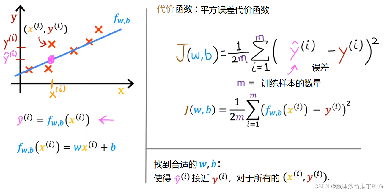
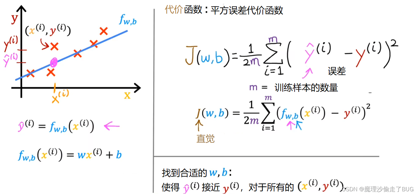
We can rewrite the cost function J of wb as 1 over 2m times the sum from i equals 1 to m of f of x^i minus y^i the quantity squared.
我們可以將損失函數 J ( w , b ) J(w,b) J(w,b)重寫為 J ( w , b ) = 1 2 m ∑ i = 1 m ( f ( x ( i ) ) ? y ( i ) ) 2 J(w,b)=\frac{1}{2m}\displaystyle \sum_{i=1}^{m} \left(f(x^{(i)})-y^{(i)}\right)^2 J(w,b)=2m1?i=1∑m?(f(x(i))?y(i))2
Eventually we’re going to want to find values of w and b that make the cost function small.
最后,我們要找到使代價函數最小的 w w w和 b b b.
But before going there, let’s first gain more intuition about what J of wb is really computing.
在深入探討之前,讓我們首先更好地理解 J ( w , b ) J(w,b) J(w,b)到底在計算什么。
At this point you might be thinking we’ve done a whole lot of math to define the cost function. But what exactly is it doing? Let’s go on to the next video where we’ll step through one example of what the cost function is really computing that I hope will help you build intuition about what it means if J of wb is large versus if the cost j is small. Let’s go on to the next video.
到目前為止,你可能正在想我們已經進行了很多數學推導來定義代價函數。但是,它到底是在做什么呢?讓我們繼續看下一個視頻,在下一個視頻中,我們將通過一個例子詳細解釋損失函數到底在計算什么,希望能幫助你對 J ( w , b ) J(w,b) J(w,b)的大或小的含義建立直覺。讓我們繼續觀看下一個視頻。

密碼加密網絡安全)


))詳細介紹】)


