目錄
- 平滑(低通)空間濾波器
- 低通高斯濾波器核
- 統計排序(非線性)濾波器
平滑(低通)空間濾波器
平滑(也稱平均)空間濾波器用于降低灰度的急劇過渡
- 在圖像重取樣之前平滑圖像以減少混淆
- 用于減少圖像中無關細節
- 平滑因灰度級數量不足導致的圖像中的偽輪廓
- 平滑核與一幅圖像的卷積會模糊圖像
低通高斯濾波器核
高斯核是唯一可分離的圓對稱(也稱各向同性,意味它們的響應與方向無關)核。
w(s,t)=G(s,t)=Ke?s2+t22σ2(3.45)w(s,t) = G(s,t) = K e^{-\frac{s^2 + t^2}{2\sigma^2}} \tag{3.45}w(s,t)=G(s,t)=Ke?2σ2s2+t2?(3.45)
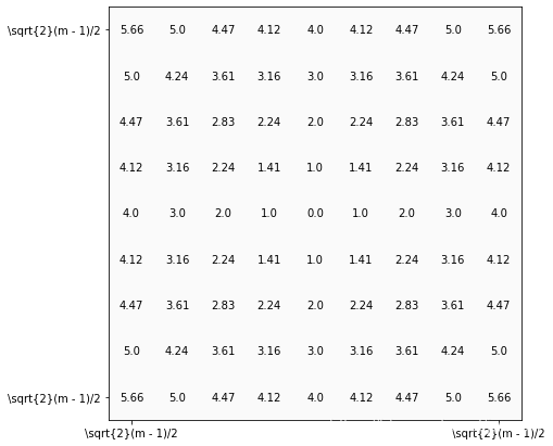
令r=[s2+t2]1/2r = [s^2 + t^2]^{1/2}r=[s2+t2]1/2,上式可以重寫為
G(r)=Ke?r22σ2(3.46)G(r) = K e^{-\frac{r^2}{2\sigma^2}} \tag{3.46}G(r)=Ke?2σ2r2?(3.46)
高斯分布函數
G(x)=12πσe?(x?x0)22σ2G(x) = \frac{1}{\sqrt{2\pi\sigma}}e^{-\frac{(x-x_0)^2}{2\sigma^2}}G(x)=2πσ?1?e?2σ2(x?x0?)2?
G(x,y)=12πσ2e?(x?x0)2+(y?y0)22σ2G(x, y) = \frac{1}{2\pi\sigma^2}e^{-\frac{(x-x_0)^2+(y-y_0)^2}{2\sigma^2}}G(x,y)=2πσ21?e?2σ2(x?x0?)2+(y?y0?)2?
3X3高斯核:
14.897?[0.36790.60650.36790.606510.60650.36790.60650.3679]\frac{1}{4.897} *\begin{bmatrix} 0.3679 & 0.6065 & 0.3679 \\ 0.6065 & 1 & 0.6065\\ 0.3679 & 0.6065 & 0.3679 \end{bmatrix}4.8971?????0.36790.60650.3679?0.606510.6065?0.36790.60650.3679????
下面的近似高斯核(效果很接近)
116?[121242121]\frac{1}{16} *\begin{bmatrix} 1& 2& 1 \\ 2& 4& 2 \\ 1& 2& 1\end{bmatrix}161?????121?242?121????
1273?[1474141626164726412674162616414741]\frac{1}{273} * \begin{bmatrix} 1& 4& 7& 4& 1 \\ 4& 16& 26& 16& 4 \\ 7& 26& 41& 26& 7 \\ 4& 16& 26& 16& 4 \\ 1& 4& 7&4&1\end{bmatrix}2731?????????14741?41626164?72641267?41626164?14741????????
下面是兩種方式構建低通高斯濾波器核
def gauss_seperate_kernel(kernel_size, sigma=1):"""create gaussian kernel use separabal vector, because gaussian kernel is symmetric and separable.param: kernel_size: input, the kernel size you want to create, normally is uneven number, such as 1, 3, 5, 7param: sigma: input, sigma of the gaussian fuction, default is 1return a desired size 2D gaussian kernel"""if sigma == 0:sigma = ((kernel_size - 1) * 0.5 - 1) * 0.3 + 0.8m = kernel_size[0]n = kernel_size[1]x_m = np.arange(m) - m // 2y_m = np.exp(-(x_m **2 )/ (2 * sigma**2)).reshape(-1, 1)x_n = np.arange(n) - n // 2y_n = np.exp(-(x_n ** 2)/ (2 * sigma**2)).reshape(-1, 1)kernel = y_m * y_n.Treturn kernel
# gaussian kernel
gauss_seperate_kernel((5, 5)).round(3)
array([[0.018, 0.082, 0.135, 0.082, 0.018],[0.082, 0.368, 0.607, 0.368, 0.082],[0.135, 0.607, 1. , 0.607, 0.135],[0.082, 0.368, 0.607, 0.368, 0.082],[0.018, 0.082, 0.135, 0.082, 0.018]])
def gauss_kernel(kernel_size, sigma=1):"""create gaussian kernel use meshgrid, gaussian is circle symmetric.param: kernel_size: input, the kernel size you want to create, normally is uneven number, such as 1, 3, 5, 7param: sigma: input, sigma of the gaussian fuction, default is 1return a desired size 2D gaussian kernel"""
#     X = np.arange(-kernel_size // 2 +1, kernel_size//2 +1)
#     Y = np.arange(-kernel_size // 2 +1, kernel_size//2 +1)m = kernel_size[0]n = kernel_size[1]X = np.arange(- m//2 + 1, m//2+1)Y = np.arange(- n//2 + 1, n//2+1)x, y = np.meshgrid(X, Y)kernel = np.exp(- ((x)**2 + (y)**2)/ (2 * sigma**2))return kernel
# gaussian kernel
gauss_kernel((5, 5)).round(3)
array([[0.018, 0.082, 0.135, 0.082, 0.018],[0.082, 0.368, 0.607, 0.368, 0.082],[0.135, 0.607, 1. , 0.607, 0.135],[0.082, 0.368, 0.607, 0.368, 0.082],[0.018, 0.082, 0.135, 0.082, 0.018]])
def visualize_show_annot(img_show, img_annot, ax):"""add annotation to the image, values of each pixelparam: img: input imageparam: ax: axes of the matplotlib"""height, width = img_annot.shapeimg_show = img_show[:height, :width]ax.imshow(img_show, cmap='gray', vmin=0, vmax=255)thresh = 10 #img_show.max()/2.5for x in range(height):for y in range(width):ax.annotate(str(round(img_annot[x][y],2)), xy=(y,x),horizontalalignment='center',verticalalignment='center',color='white' if img_annot[x][y]>thresh else 'black')
# 顯示距離
m = 9
S = np.arange(- (m - 1) // 2, (m - 1) // 2 + 1)
T = S
s, t = np.meshgrid(S, T)
r = np.power((s**2 + t**2), 0.5)height, width = m, m
img_show = np.ones([height, width], dtype=np.uint8) * 250
fig = plt.figure(figsize=(7, 7))
ax = fig.add_subplot(1, 1, 1)
visualize_show_annot(img_show, r, ax)
plt.xticks([0, m-1], labels=["\sqrt{2}(m - 1)/2", "\sqrt{2}(m - 1)/2"]) # 標簽顯示不了\sqrt{2},所以簡寫(m-1)/2
ax.set_yticks([0, m-1])
ax.set_yticklabels(["\sqrt{2}(m - 1)/2", "\sqrt{2}(m - 1)/2"])
plt.show()
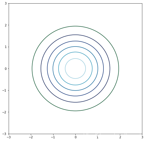
# 顯示高斯核濾波器的圓
import numpy as np
import mpl_toolkits.mplot3d
from matplotlib import pyplot as plt
from matplotlib import cmx, y = np.mgrid[-3:3:200j,-3:3:200j]
z = np.exp(- ((x)**2 + (y)**2)/ (2))fig = plt.figure(figsize=(8,8))
ax = fig.gca()
ax.contour(x, y, z, cmap=cm.ocean)
plt.show()
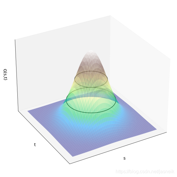
# 二維高斯核函數
from mpl_toolkits.mplot3d import Axes3D
import numpy as np
from matplotlib import pyplot as pltk = 3
sigma = 1
X = np.linspace(-k, k, 100)
Y = np.linspace(-k, k, 100)
x, y = np.meshgrid(X, Y)
z = np.exp(- ((x)**2 + (y)**2)/ (2 * sigma**2))fig = plt.figure(figsize=(8, 8))
ax = Axes3D(fig)
ax.set_xticks([])
ax.set_yticks([])
ax.set_zticks([])
ax.set_xlabel('s', fontsize=14)
ax.set_ylabel('t', fontsize=14)
ax.set_zlabel('G(s,t)', fontsize=14)
ax.plot_surface(x, y, z, antialiased=True, shade=False, alpha=0.5, cmap=cm.terrain)
ax.contour(x, y, z, [0.3, 0.6], colors='k')
ax.view_init(30, 60)
plt.show()
兩個一維高斯函數fff和ggg和乘積(×\times×)和卷積(?\star?)的均值與標準差
| fff | ggg | f×gf\times{g}f×g | f?gf\star{g}f?g | |
|---|---|---|---|---|
| 均值 | mfm_fmf? | mgm_gmg? | mf×g=mfσg2+mgσf2σf2+σg2m_{f\times{g}}=\frac{m_{f} \sigma_{g}^2 + m_{g} \sigma_{f}^2}{\sigma_{f}^2 + \sigma_{g}^2}mf×g?=σf2?+σg2?mf?σg2?+mg?σf2?? | mf?g=mf+mgm_{f\star{g}} = m_{f} + m_{g}mf?g?=mf?+mg? |
| 標準差 | σf\sigma_{f}σf? | σg\sigma_{g}σg? | σf×g=σf2σg2σf2+σg2\sigma_{f\times{g}}=\sqrt{\frac{\sigma_{f}^2 \sigma_{g}^2}{\sigma_{f}^2 + \sigma_{g}^2}}σf×g?=σf2?+σg2?σf2?σg2??? | σf?g=σf2+σg2\sigma_{f\star{g}} = \sigma_{f}^2 + \sigma_{g}^2σf?g?=σf2?+σg2? |
# 高斯核生成函數 之前沒有怎么看書的時候寫的,不太正確
def creat_gauss_kernel(kernel_size=3, sigma=1, k=1):if sigma == 0:sigma = ((kernel_size - 1) * 0.5 - 1) * 0.3 + 0.8X = np.linspace(-k, k, kernel_size)Y = np.linspace(-k, k, kernel_size)x, y = np.meshgrid(X, Y)x0 = 0y0 = 0gauss = 1/(2*np.pi*sigma**2) * np.exp(- ((x -x0)**2 + (y - y0)**2)/ (2 * sigma**2))##繪圖功能
#     fig = plt.figure(figsize=(8,6))
#     ax = fig.gca(projection='3d')
#     ax.plot_surface(x,y,gauss,cmap=plt.cm.ocean)
#     plt.show()return gauss
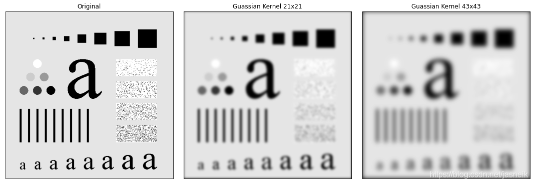
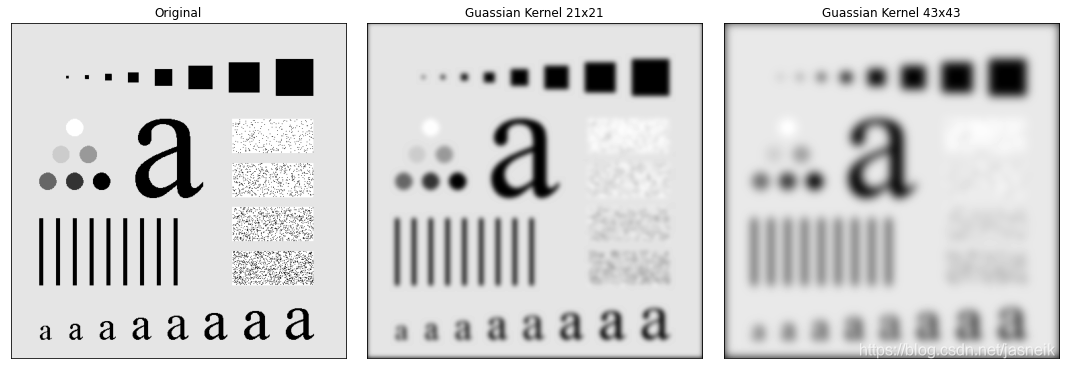
#不同的大小,不同sigma的高斯核
img_gray = cv2.imread('DIP_Figures/DIP3E_Original_Images_CH03/Fig0333(a)(test_pattern_blurring_orig).tif', 0)
kernel_21 = gauss_kernel((21, 21), sigma=3.5)
kernel_21 = kernel_21 / kernel_21.sum()
kernel_43 = gauss_kernel((43, 43), sigma=7)
kernel_43 = kernel_43 / kernel_43.sum()
# img_21 = cv2.filter2D(img_gray, ddepth= -1, kernel=kernel_21)
# img_43 = cv2.filter2D(img_gray, ddepth= -1, kernel=kernel_43)
img_21 = my_conv2d(img_gray, kernel=kernel_21)
img_43 = my_conv2d(img_gray, kernel=kernel_43)plt.figure(figsize=(15, 5))
plt.subplot(1, 3, 1), plt.imshow(img_gray, cmap='gray', vmin=0, vmax=255), plt.title(f'Original')
plt.xticks([]), plt.yticks([])
plt.subplot(1, 3, 2), plt.imshow(img_21, cmap='gray', vmin=0, vmax=255), plt.title(f'Gaussian Kernel 21x21')
plt.xticks([]), plt.yticks([])
plt.subplot(1, 3, 3), plt.imshow(img_43, cmap='gray', vmin=0, vmax=255), plt.title(f'Gaussian Kernel 43x43')
plt.xticks([]), plt.yticks([])
plt.tight_layout()
plt.show()
#不同的大小,不同sigma的高斯核,用可分離核運算的話,高斯核不用歸一化,但計算后歸一化后再乘以255
img_gray = cv2.imread('DIP_Figures/DIP3E_Original_Images_CH03/Fig0333(a)(test_pattern_blurring_orig).tif', 0)
kernel_21 = gauss_kernel((21, 21), sigma=3.5)
# kernel_21 = kernel_21 / kernel_21.sum()
kernel_43 = gauss_kernel((43, 43), sigma=7)
# kernel_43 = kernel_43 / kernel_43.sum()
img_21 = separate_kernel_conv2D(img_gray, kernel=kernel_21)
img_21 = np.uint8(normalize(img_21) * 255)
img_43 = separate_kernel_conv2D(img_gray, kernel=kernel_43)
img_43 =  np.uint8(normalize(img_43) * 255)
plt.figure(figsize=(15, 5))
plt.subplot(1, 3, 1), plt.imshow(img_gray, cmap='gray', vmin=0, vmax=255), plt.title(f'Original')
plt.xticks([]), plt.yticks([])
plt.subplot(1, 3, 2), plt.imshow(img_21, cmap='gray', vmin=0, vmax=255), plt.title(f'Gaussian Kernel 21x21')
plt.xticks([]), plt.yticks([])
plt.subplot(1, 3, 3), plt.imshow(img_43, cmap='gray', vmin=0, vmax=255), plt.title(f'Gaussian Kernel 43x43')
plt.xticks([]), plt.yticks([])
plt.tight_layout()
plt.show()
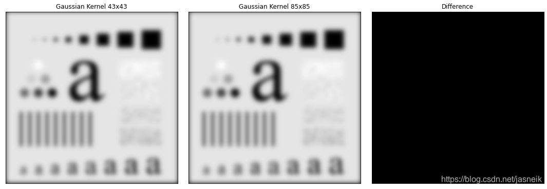
#大于[6sigma] x [6sigma]的高斯核并無益處,由于opencv返回的圖像都是uint8的,從差來看,還是有點區別,但是兩者的結果視覺上看差不多
#用自己實現的卷積,返回的是float,結果的最大值為0.948,比opencv的效果好,就是執行的效率不高,opencv計算是相關性,而不是真的卷積運算
img_gray = cv2.imread('DIP_Figures/DIP3E_Original_Images_CH03/Fig0333(a)(test_pattern_blurring_orig).tif', 0)kernel_43 = gauss_kernel((43, 43), sigma=7)
kernel_43 = kernel_43 / kernel_43.sum()
# img_43 = cv2.filter2D(img_gray, ddepth= -1, kernel=kernel_43)
img_43 = my_conv2d(img_gray, kernel=kernel_43)kernel_85 = gauss_kernel((85, 85), sigma=7)
kernel_85 = kernel_85 / kernel_85.sum()
# img_85 = cv2.filter2D(img_gray, ddepth= -1, kernel=kernel_85)
img_85 = my_conv2d(img_gray, kernel=kernel_85)img_diff = img_85 - img_43
plt.figure(figsize=(15, 5))
plt.subplot(1, 3, 1), plt.imshow(img_43, cmap='gray', vmin=0, vmax=255), plt.title(f'Gaussian Kernel 43x43')
plt.xticks([]), plt.yticks([])
plt.subplot(1, 3, 2), plt.imshow(img_85, cmap='gray', vmin=0, vmax=255), plt.title(f'Gaussian Kernel 85x85')
plt.xticks([]), plt.yticks([])
plt.subplot(1, 3, 3), plt.imshow(img_diff, cmap='gray', vmin=0, vmax=255), plt.title(f'Difference')
plt.xticks([]), plt.yticks([])
plt.tight_layout()
plt.show()
def down_sample(image):height, width = image.shape[:2]dst = np.zeros([height//2, width//2])dst = image[::2, ::2]return dst
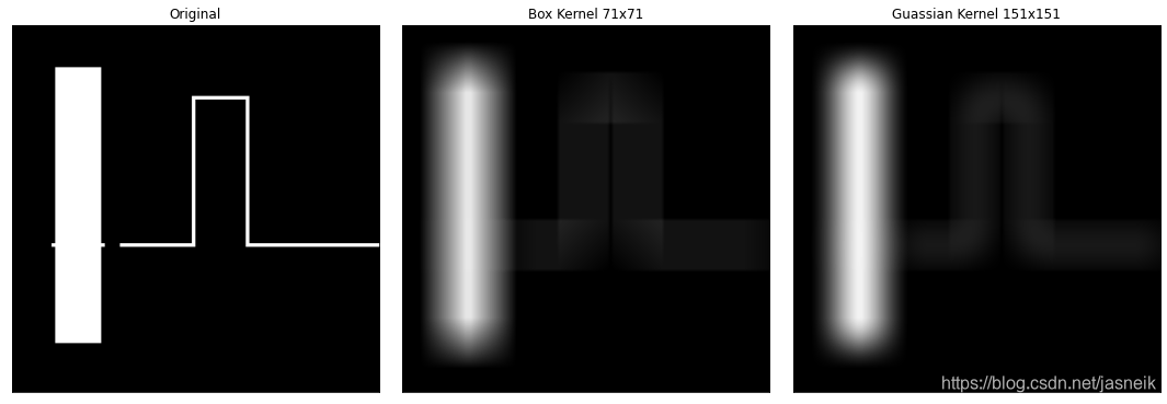
#高斯核與盒式平滑特性的比較,圖像原尺寸為1024,但報內錯誤,做降采樣,可以運行了。
#矩形區域為768x128,線的寬度為10,
height, width = 1024, 1024
img_ori = np.zeros([height, width], np.uint8)
shift = 120
img_ori[shift:shift+768, shift:shift+128] = 255
img_ori[610:620, 110:258] = 255   # 矩形背后的橫線
img_ori[610:620, 300:500] = 255   #橫線
img_ori[200:620, 500:510] = 255   #豎線
img_ori[200:210, 510:660] = 255   #橫線
img_ori[210:620, 650:660] = 255   #豎線
img_ori[610:620, 660:]    = 255   #橫線# 做降采樣縮小圖像可以不報錯了
img_ori = down_sample(img_ori)
# 盒式濾波器核 35x35,書上是71x71
box_71 = np.ones([71, 71], np.float)
box_71 = box_71 / box_71.sum()
# 高斯濾波器核71x71,書上要求是151x151,但會報內存錯誤
gauss_151 = gauss_kernel((71, 71), sigma=25)
gauss_151 = gauss_151 / gauss_151.sum()
img_box_71 = my_conv2d(img_ori, kernel=box_71)
img_gauss_151 = my_conv2d(img_ori, kernel=gauss_151)# # # opencv處理線都不見了,不是真的做卷積運算
# # img_box_71 = cv2.filter2D(img_ori, ddepth=-1, kernel=box_71)
# # img_gauss_151 = cv2.filter2D(img_ori, ddepth=-1, kernel=gauss_151)plt.figure(figsize=(15, 5))
plt.subplot(1, 3, 1), plt.imshow(img_ori, cmap='gray', vmin=0, vmax=255), plt.title(f'Original')
plt.xticks([]), plt.yticks([])
plt.subplot(1, 3, 2), plt.imshow(img_box_71, cmap='gray', vmin=0, vmax=255), plt.title(f'Box Kernel 71x71')
plt.xticks([]), plt.yticks([])
plt.subplot(1, 3, 3), plt.imshow(img_gauss_151, cmap='gray', vmin=0, vmax=255), plt.title(f'gaussian Kernel 151x151')
plt.xticks([]), plt.yticks([])
plt.tight_layout()
plt.show()
def nomalize(img):return (img - img.min()) / (img.max() - img.min())
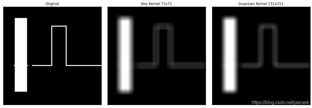
#高斯核與盒式平滑特性的比較,圖像原尺寸為1024,用可分離核計算1024,也不會報錯的。
#矩形區域為768x128,線的寬度為10,
height, width = 1024, 1024
img_ori = np.zeros([height, width], np.uint8)
shift = 120
img_ori[shift:shift+768, shift:shift+128] = 255
img_ori[610:620, 110:258] = 255   # 矩形背后的橫線
img_ori[610:620, 300:500] = 255   #橫線
img_ori[200:620, 500:510] = 255   #豎線
img_ori[200:210, 510:660] = 255   #橫線
img_ori[210:620, 650:660] = 255   #豎線
img_ori[610:620, 660:]    = 255   #橫線# 做降采樣縮小圖像可以不報錯了
# img_ori = down_sample(img_ori)
# 盒式濾波器核 35x35,書上是71x71
box_71 = np.ones([71, 71], np.float)
box_71 = box_71 / box_71.sum()
# 高斯濾波器核71x71,書上要求是151x151,但會報內存錯誤
gauss_151 = gauss_kernel((71, 71), sigma=25)
gauss_151 = gauss_151 / gauss_151.sum()
img_box_71 = separate_kernel_conv2D(img_ori, kernel=box_71)
img_box_71 = np.uint8(nomalize(img_box_71) * 255)
img_gauss_151 = separate_kernel_conv2D(img_ori, kernel=gauss_151)
img_gauss_151 = np.uint8(nomalize(img_gauss_151) * 255)
# # # opencv處理線都不見了,不是真的做卷積運算
# # img_box_71 = cv2.filter2D(img_ori, ddepth=-1, kernel=box_71)
# # img_gauss_151 = cv2.filter2D(img_ori, ddepth=-1, kernel=gauss_151)plt.figure(figsize=(15, 5))
plt.subplot(1, 3, 1), plt.imshow(img_ori, cmap='gray', vmin=0, vmax=255), plt.title(f'Original')
plt.xticks([]), plt.yticks([])
plt.subplot(1, 3, 2), plt.imshow(img_box_71, cmap='gray', vmin=0, vmax=255), plt.title(f'Box Kernel 71x71')
plt.xticks([]), plt.yticks([])
plt.subplot(1, 3, 3), plt.imshow(img_gauss_151, cmap='gray', vmin=0, vmax=255), plt.title(f'gaussian Kernel 151x151')
plt.xticks([]), plt.yticks([])
plt.tight_layout()
plt.show()
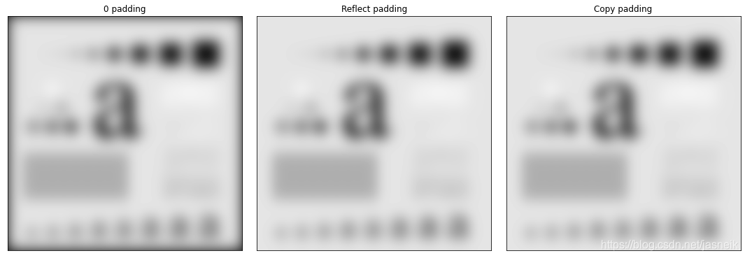
#相同的核,不同的邊填充對結果的邊的影響
img_gray = cv2.imread('DIP_Figures/DIP3E_Original_Images_CH03/Fig0333(a)(test_pattern_blurring_orig).tif', 0)# kernel size is 111x111, sigma=31,核太大了,計算會消耗很大的內存
kernel_111 = guass_kernel((111, 111), sigma=15)
kernel_111 = kernel_111 / kernel_111.sum()img_constant = my_conv2d(img_gray, kernel=kernel_111, mode='constant')
img_reflect = my_conv2d(img_gray, kernel=kernel_111, mode='reflect')
img_copy = my_conv2d(img_gray, kernel=kernel_111, mode='edge')plt.figure(figsize=(15, 5))
plt.subplot(1, 3, 1), plt.imshow(img_constant, cmap='gray', vmin=0, vmax=255), plt.title(f'0 padding')
plt.xticks([]), plt.yticks([])
plt.subplot(1, 3, 2), plt.imshow(img_reflect, cmap='gray', vmin=0, vmax=255), plt.title(f'Reflect padding')
plt.xticks([]), plt.yticks([])
plt.subplot(1, 3, 3), plt.imshow(img_copy, cmap='gray', vmin=0, vmax=255), plt.title(f'Copy padding')
plt.xticks([]), plt.yticks([])
plt.tight_layout()
plt.show()
def up_sample_2d(img):"""up sample 2d image, if your image is RGB, you could up sample each channel, then use np.dstack to merge a RGB imageparam: input img: it's a 2d gray imagereturn a 2x up sample image"""height, width = img.shape[:2]temp = np.zeros([height*2, width*2])temp[::2, ::2] = imgtemp[1::2, 1::2] = imgtemp[0::2, 1::2] = imgtemp[1::2, 0::2] = imgreturn temp
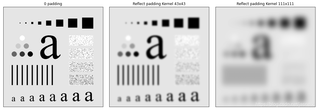
#核和圖像大小對平滑性能的影響
img_gray = cv2.imread('DIP_Figures/DIP3E_Original_Images_CH03/Fig0333(a)(test_pattern_blurring_orig).tif', 0)# 原圖像是500x500,結果兩次上采樣,變是2000x2000
img_up = up_sample_2d(img_gray)
# img_up = up_sample_2d(img_up)# 本想要升到2000x2000再做卷積,但報內存錯誤,只好試1000x1000的了
kernel_43 = guass_kernel((43, 43), sigma=7)
kernel_43 = kernel_43 / kernel_43.sum()
img_43 = my_conv2d(img_up, kernel=kernel_43, mode='reflect')# kernel size is 111x111, sigma=31,核太大了,計算會消耗很大的內存
kernel_111 = guass_kernel((111, 111), sigma=15)
kernel_111 = kernel_111 / kernel_111.sum()
img_111 = my_conv2d(img_gray, kernel=kernel_111, mode='reflect')plt.figure(figsize=(15, 5))
plt.subplot(1, 3, 1), plt.imshow(img_gray, cmap='gray', vmin=0, vmax=255), plt.title(f'0 padding')
plt.xticks([]), plt.yticks([])
plt.subplot(1, 3, 2), plt.imshow(img_43, cmap='gray', vmin=0, vmax=255), plt.title(f'Reflect padding Kernel 43x43')
plt.xticks([]), plt.yticks([])
plt.subplot(1, 3, 3), plt.imshow(img_111, cmap='gray', vmin=0, vmax=255), plt.title(f'Reflect padding Kernel 111x111')
plt.xticks([]), plt.yticks([])
plt.tight_layout()
plt.show()
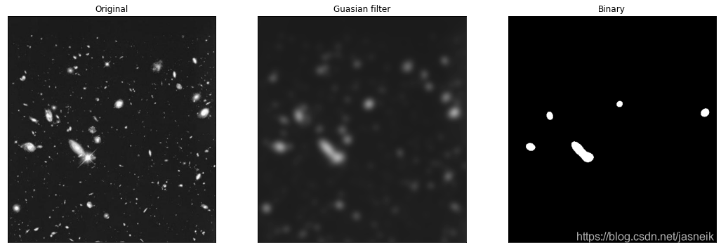
#使用低通濾波和閾值處理提取區域,根據自己的要求要選擇核的大小
img_ori = cv2.imread('DIP_Figures/DIP3E_Original_Images_CH03/Fig0334(a)(hubble-original).tif', 0)
img_ori = img_ori / 255.kernel_43 = gauss_kernel((43, 43), sigma=7)
kernel_43 = kernel_43 / kernel_43.sum()
img_43 = my_conv2d(img_ori, kernel=kernel_43, mode='reflect')thred = 0.42
img_thred = np.where(img_43 <= thred, img_43, 1)
img_thred = np.where(img_43 > thred, img_thred, 0)plt.figure(figsize=(15, 5))
plt.subplot(1, 3, 1), plt.imshow(img_ori, cmap='gray', vmin=0, vmax=1), plt.title(f'Original')
plt.xticks([]), plt.yticks([])
plt.subplot(1, 3, 2), plt.imshow(img_43, cmap='gray', vmin=0, vmax=1), plt.title(f'Gaussian filter')
plt.xticks([]), plt.yticks([])
plt.subplot(1, 3, 3), plt.imshow(img_thred, cmap='gray', vmin=0, vmax=1), plt.title(f'Binary')
plt.xticks([]), plt.yticks([])
plt.tight_layout()
plt.show()
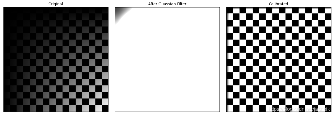
陰影校正(也稱平坦場校正)
def filter_2d(image, kernel, mode='constant'):"""convolution 2d image with kernel:param image: input image:param kernel: input kernel:return: image after convolution"""img_h = image.shape[0]img_w = image.shape[1]m = kernel.shape[0]n = kernel.shape[1]# paddingpadding_h = int((m -1)/2)padding_w = int((n -1)/2)image_pad = np.pad(image, [(padding_h, padding_h), (padding_w, padding_w)], mode=mode)
#     image_pad = np.zeros((image.shape[0]+padding_h*2, image.shape[1]+padding_w*2), np.uint8)
#     image_pad[padding_h:padding_h+img_h, padding_w:padding_w+img_w] = imageimage_convol = image.copy()for i in range(padding_h, img_h + padding_h):for j in range(padding_w, img_w + padding_w):temp = np.sum(image_pad[i-padding_h:i+padding_h+1, j-padding_w:j+padding_w+1] * kernel)image_convol[i - padding_h][j - padding_w] = temp # 1/(m * n) * tempreturn image_convol
def get_check(height, width, check_size=(5, 5), lower=130, upper=255):"""create check pattern imageheight: input, height of the image you wantwidth: input, width of the image you wantcheck_size: the check size you want, default is 5x5lower: dark color of the check, default is 130, which is dark gray, 0 is black, 255 is whiteupper: light color of the check, default is 255, which is white, 0 is blackreturn uint8[0, 255] grayscale check pattern image"""m, n = check_sizeblack = np.zeros((m, n), np.uint8)white = np.zeros((m, n), np.uint8)black[:] = lower # darkwhite[:] = upper # whiteblack_white = np.concatenate([black, white], axis=1)white_black = np.concatenate([white, black], axis=1)black_white_black_white = np.vstack((black_white, white_black))tile_times_h = int(np.ceil(height / m / 2))tile_times_w = int(np.ceil(width / n / 2))img_temp = np.tile(black_white_black_white, (tile_times_h, tile_times_w))img_dst = np.zeros([height, width])img_dst = img_temp[:height, :width]return img_dst
def get_shape_pattern(img_ori):"""create a dark mask shape of the imageimg_ori: input image, which only use the image shape here to create the maskreturn [0, 1] float image"""height, width = img_ori.shapeimg_dst = np.zeros([height, width])for i in range(height):temp = np.linspace(0, i/width, height)img_dst[i, :] = tempimg_dst = normalize(img_dst)return img_dst
#使用低通濾波校正陰影,大核太慢了,還是用opencv的快
#創建棋盤格
height, width = 2048, 2048
img_ori = get_check(height, width, check_size=(128, 128), lower=0)#得到棋盤格圖像對應的掩膜
img_shape = get_shape_pattern(img_ori)#生成帶遮照的圖像
img_ori = img_ori * img_shape#生成513x513的高斯濾波器核
kernel_513 = guass_kernel((511, 511), sigma=128)
kernel_513 = kernel_513 / kernel_513.sum()#卷積,別用注釋掉的,按書上說的得2個小時,我也沒有試過
# img_513 = filter_2d(img_ori, kernel=kernel_513)
img_513 = cv2.filter2D(img_ori, ddepth=-1, kernel=kernel_513)#得到校正后的圖像
img_dst = img_ori / (img_513 + 1e-5)plt.figure(figsize=(15, 5))
plt.subplot(1, 3, 1), plt.imshow(img_ori, cmap='gray', vmin=0, vmax=255), plt.title(f'Original')
plt.xticks([]), plt.yticks([])
plt.subplot(1, 3, 2), plt.imshow(img_513, cmap='gray', vmin=0, vmax=1), plt.title(f'After Guassian Filter')
plt.xticks([]), plt.yticks([])
plt.subplot(1, 3, 3), plt.imshow(img_dst, cmap='gray', vmin=0, vmax=1), plt.title(f'Calibrated')
plt.xticks([]), plt.yticks([])
plt.tight_layout()
plt.show()
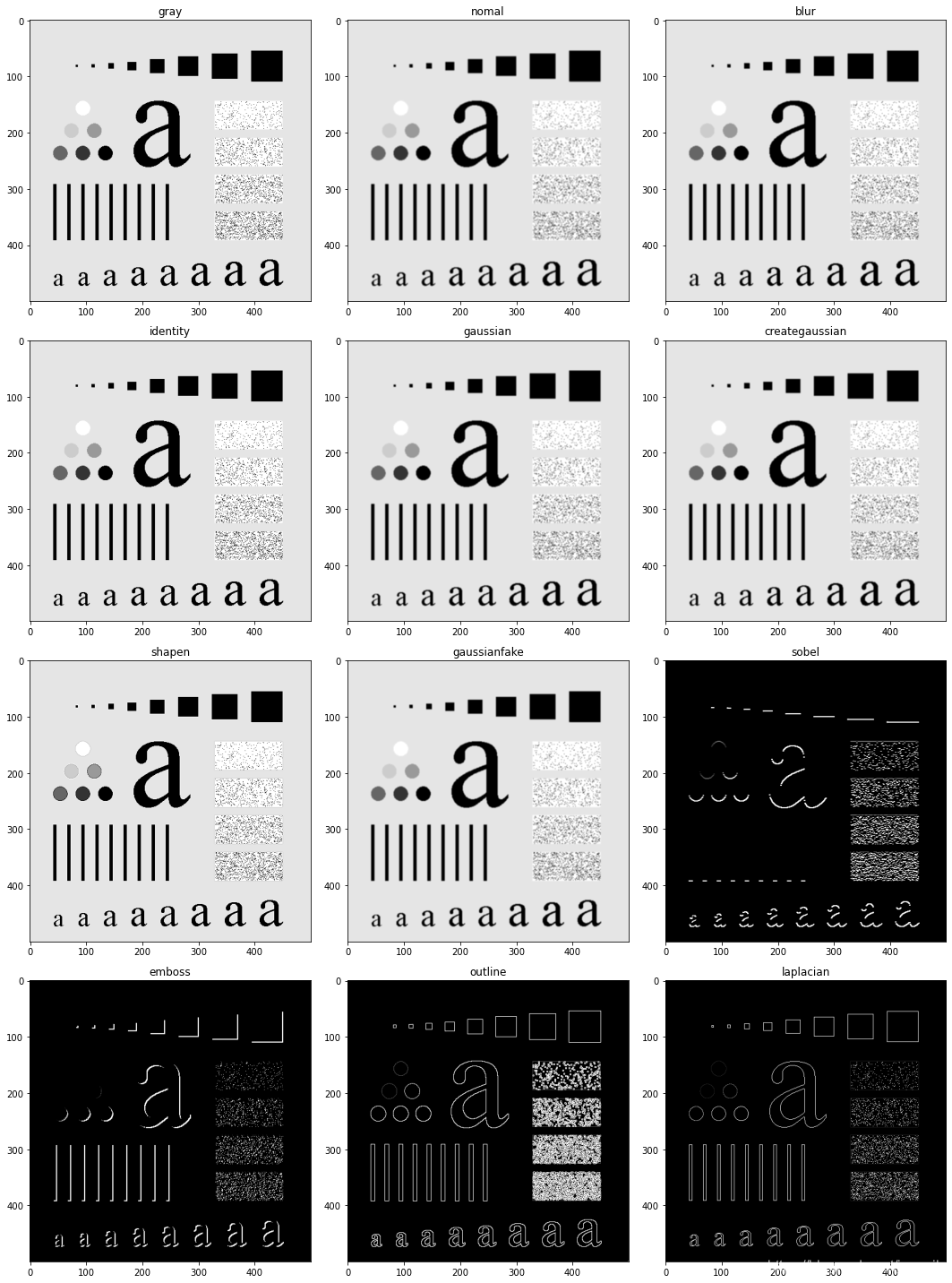
# 多種濾波器核
img = cv2.imread('DIP_Figures/DIP3E_Original_Images_CH03/Fig0333(a)(test_pattern_blurring_orig).tif')
img_gray = cv2.cvtColor(img, cv2.COLOR_BGR2GRAY)# 盒式濾波器核
kernel_normal = np.array([[1, 1, 1],[1, 1, 1],[1, 1, 1]], dtype='float32')
kernel_normal = kernel_normal / kernel_normal.sum()# 模糊算子
kernal_blur = np.array(([0.0625, 0.125, 0.0625],[0.125, 0.25, 0.125],[0.0625, 0.125, 0.0625]), dtype="float32")
kernal_blur = kernal_blur / kernal_blur.sum()# sobel算子,sobel內核用于僅顯示特定方向上相鄰像素值的差異,分為left sobel、right sobel(檢測梯度的水平變化)、top sobel、buttom sobel(檢測梯度的垂直變化)。
kernel_sobel = np.array(([-1,-2,-1],[0,0,0],[1,2,1]), np.int8)
# 浮雕算子,通過強調像素的差在給定方向的Givens深度的錯覺。在這種情況下,沿著從左上到右下的直線的方向。
kernel_emboss = np.array(([-2,-1,0],[-1,1,1],[0,-1,2]), np.int8)# 輪廓內核(也稱為“邊緣”的內核)用于突出顯示的像素值大的差異。具有接近相同強度的相鄰像素旁邊的像素在新圖像中將顯示為黑色,而與強烈不同的相鄰像素相鄰的像素將顯示為白色。
kernel_outline = np.array(([-1,-1,-1],[-1,8,-1],[-1,-1,-1]), np.int8)# 銳化算子,銳化內核強調在相鄰的像素值的差異,這使圖像看起來更生動
kernel_shapen = np.array(([0,-1,0],[-1,5,-1],[0,-1,0]), np.int8)# 拉普拉期算子,用于邊緣檢對于檢測圖像中的模糊也非常有用
kernel_laplacian = np.array(([0,1,0],[1,-4,1],[0,1,0]), np.int8)# 分身算子,就是原圖
kernel_identity = np.array(([0,0,0],[0,1,0],[0,0,0]), np.int8)# 網上找的高斯核
kernel_gaussianfake = np.array([[1, 2, 1],[2, 4, 2],[1, 2, 1]])/16
# DIP書上給了的高斯核
kernel_gaussian = np.array([[0.3679, 0.6065, 0.3679],[0.6065, 1, 0.6065],[0.3679, 0.6065, 0.3679]], np.float32) / 4.8976# 自己通過高期函數算出的高斯核
kernel_creategaussian = guass_kernel((3, 3))
kernel_creategaussian = kernel_creategaussian / kernel_creategaussian.sum()img_nomal = cv2.filter2D(img_gray, ddepth= -1, kernel=kernel_normal)
imgkernal_blur = cv2.filter2D(img_gray, -1, kernal_blur)
imgkernel_sobel = cv2.filter2D(img_gray, -1, kernel_sobel)
imgkernel_emboss = cv2.filter2D(img_gray, -1, kernel_emboss)
imgkernel_outline = cv2.filter2D(img_gray, -1, kernel_outline)
imgkernel_shapen = cv2.filter2D(img_gray, -1, kernel_shapen)
imgkernel_laplacian = cv2.filter2D(img_gray, -1, kernel_laplacian)
imgkernel_identity = cv2.filter2D(img_gray, -1, kernel_identity)
imgkernel_gaussianfake = cv2.filter2D(img_gray, -1, kernel_gaussianfake)
imgkernel_gaussian = cv2.filter2D(img_gray, -1, kernel_gaussian)
imgkernel_creategaussian = cv2.filter2D(img_gray, -1, kernel_creategaussian)
img_list = ['img_gray', 'img_nomal', 'imgkernal_blur', 'imgkernel_identity', 'imgkernel_gaussian', 'imgkernel_creategaussian', 'imgkernel_shapen', 'imgkernel_gaussianfake', 'imgkernel_sobel', 'imgkernel_emboss', 'imgkernel_outline', 'imgkernel_laplacian', ]fig = plt.figure(figsize=(15, 20))for i, img in enumerate(img_list):ax = fig.add_subplot(4, 3, i+1)ax.imshow(locals()[img], cmap='gray')ax.set_title(img.split('_')[-1])plt.tight_layout()
plt.show()
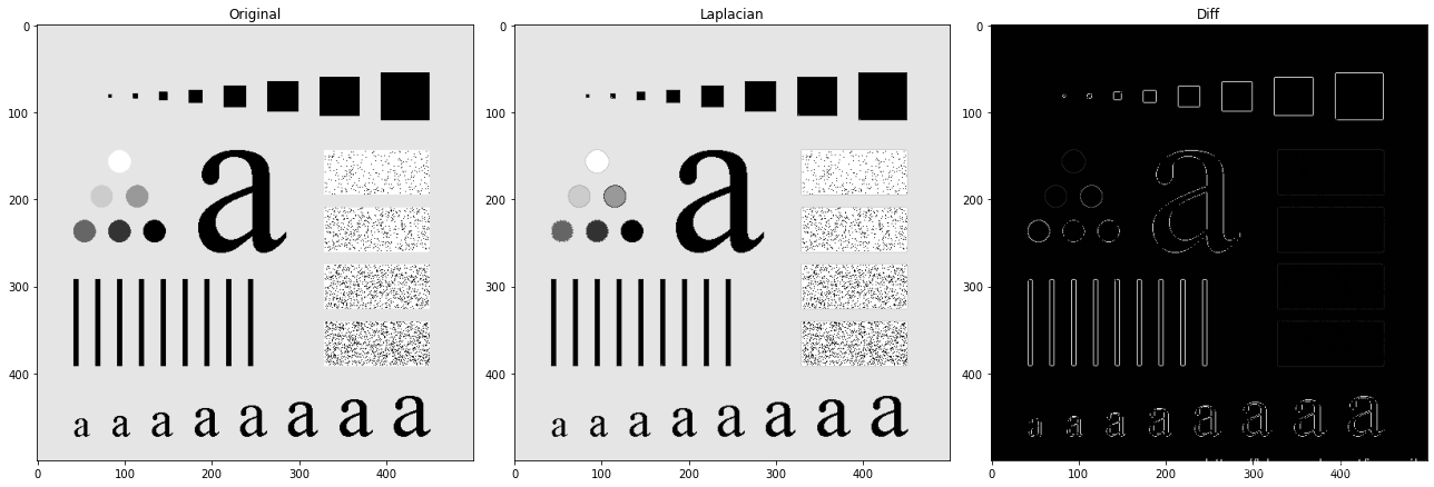
# 拉普拉斯算子銳化
laplacian_img = np.uint8(normalize(img_gray - imgkernel_laplacian) * 255)plt.figure(figsize=(18, 6))
plt.subplot(1, 3, 1)
plt.imshow(img_gray, cmap='gray')
plt.title('Original')plt.subplot(1, 3, 2)
plt.imshow(laplacian_img, cmap='gray')
plt.title('Laplacian')img_diff = img_gray - laplacian_img
plt.subplot(1, 3, 3)
plt.imshow(img_diff, cmap='gray')
plt.title('Diff')
plt.tight_layout()
plt.show()
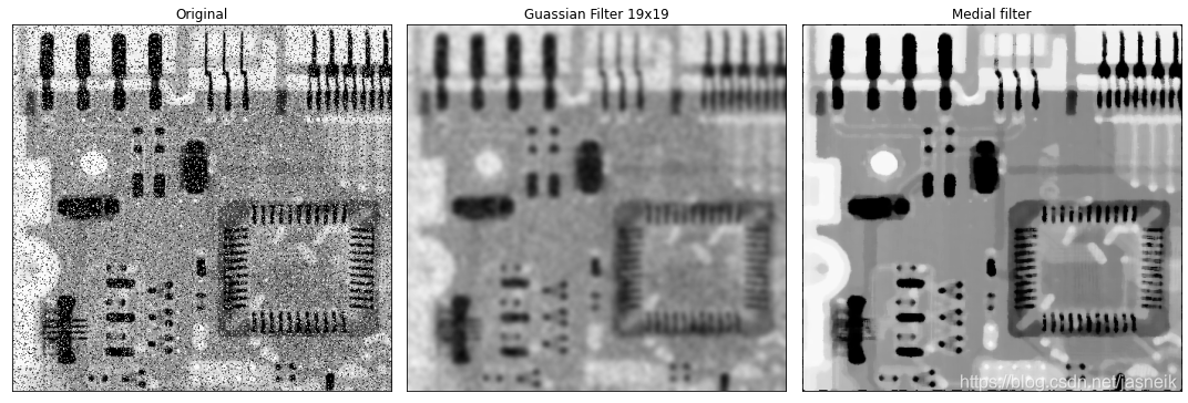
統計排序(非線性)濾波器
統計排序濾波器是非線性空間濾波器,其響應基于濾波器所包含區域內的像素的排序。平滑是將中心像素的值替代為由排序結果確定的值來實現的。
- 中值濾波器
- 中值濾波器對某些類型的隨機噪聲提供了優秀的降噪能力
- 與類似大小的線性平滑濾波器相對,中值濾波器對圖像的模糊程度要小得多。
- 對椒鹽噪聲尤其有效
- 鄰域內的中值
def median_filter(img, kernel_size, mode="constant"):"""median filterparam: img: input image for denoisingparam: kernel_size: kernel size of the median filter blockreturn: image after median filter"""img_h = img.shape[0]img_w = img.shape[1]m = kernel_size[0]n = kernel_size[1]pad_h = int((m - 1)/2)pad_w = int((n - 1)/2)# 邊界通過0灰度值填充擴展img_pad = np.pad(img, [(pad_h, pad_h), (pad_w, pad_w)], mode=mode)img_result = np.zeros(img.shape)for i in range(img_result.shape[0]):for j in range(img_result.shape[1]):temp = img_pad[i:i + m, j:j + n]img_result[i, j] = np.median(temp)return img_result
# 中值濾波器與高斯低通濾波器比較
img_ori = cv2.imread('DIP_Figures/DIP3E_Original_Images_CH03/Fig0335(a)(ckt_board_saltpep_prob_pt05).tif', 0)kernel_19 = guass_kernel((19, 19), sigma=3)
kernel_19 = kernel_19 / kernel_19.sum()img_19 = cv2.filter2D(img_ori, ddepth=-1, kernel=kernel_19)img_median = median_filter(img_ori, (7, 7), mode='constant')plt.figure(figsize=(15, 5))
plt.subplot(1, 3, 1), plt.imshow(img_ori, cmap='gray', vmin=0, vmax=255), plt.title(f'Original')
plt.xticks([]), plt.yticks([])
plt.subplot(1, 3, 2), plt.imshow(img_19, cmap='gray', vmin=0, vmax=255), plt.title(f'Guassian Filter 19x19')
plt.xticks([]), plt.yticks([])
plt.subplot(1, 3, 3), plt.imshow(img_median, cmap='gray', vmin=0, vmax=255), plt.title(f'Medial filter')
plt.xticks([]), plt.yticks([])
plt.tight_layout()
plt.show()


 - 灰度變換與空間濾波15 - 銳化高通濾波器 -拉普拉斯核(二階導數))


 - 灰度變換與空間濾波16 - 銳化高通濾波器 - 鈍化掩蔽和高提升濾波)


 - 灰度變換與空間濾波17 - 銳化高通濾波器 - 梯度圖像(羅伯特,Sobel算子))