本章主要講解頻域域濾波的技術，主要技術用到是大家熟悉的傅里葉變換與傅里葉反變換。這里有比較多的篇幅講解的傅里葉的推導進程，用到Numpy傅里葉變換。本章理論基礎比較多，需要更多的耐心來閱讀，有發現有錯誤，可以與我聯系。謝謝！

import sys
import numpy as np
import cv2
import matplotlib 
import matplotlib.pyplot as plt
import PIL
from PIL import Imageprint(f"Python version: {sys.version}")
print(f"Numpy version: {np.__version__}")
print(f"Opencv version: {cv2.__version__}")
print(f"Matplotlib version: {matplotlib.__version__}")
print(f"Pillow version: {PIL.__version__}")

Python version: 3.6.12 |Anaconda, Inc.| (default, Sep  9 2020, 00:29:25) [MSC v.1916 64 bit (AMD64)]
Numpy version: 1.16.6
Opencv version: 3.4.1
Matplotlib version: 3.3.2
Pillow version: 8.0.1

def normalize(mask):return (mask - mask.min()) / (mask.max() - mask.min() + 1e-8)

背景

傅里葉級數和變換簡史

內容比較多，請自行看書，我就實現一維的傅里葉變換先。

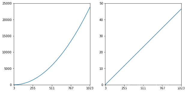
卷積用大小為$m\times n$元素的核對大小為$M\times N$的圖像進行濾波時，需要運算次數為$MNmn$。如果核是可分享的，那么運算次數為$MN(m+N)$，而在頻率域執行等交的濾波所需要的運算次數為$2MN{\text{log}}_{2}MN$，2表示計算一次正FFT和一次反FFT。

$$C_n(m)=\frac{M^2{m}^2}{2M^2{\text{log}}_2}{M}^2=\frac{m^2}{4{\text{log}}_{2}M}\text{\hspace{1em}(4.1)}$$

如果是可分離核，則變為

$$C_s(m)=\frac{M^2{m}^2}{2M^2{\text{log}}_2{M}^2}=\frac{m}{2{\text{log}}_{2}M}\text{\hspace{1em}(4.2)}$$

當$C(m)>1$時，FFT的方法計算優勢更大；而$C(m)\le 1$時，空間濾波的優勢更大

# FFT 計算的優勢
M = 2048
m = np.arange(0, 1024, 1)
c_n = m**2 / (4 * np.log2(M))
c_s = m / (2 * np.log2(M))
fig = plt.figure(figsize=(10, 5))
ax_1 = fig.add_subplot(1, 2, 1)
ax_1.plot(c_n)
ax_1.set_xlim([0, 1024])
ax_1.set_xticks([3, 255, 511, 767, 1023])
ax_1.set_ylim([0, 25*1e3])
ax_1.set_yticks([0, 5*1e3, 10*1e3, 15*1e3, 20*1e3, 25*1e3])
ax_2 = fig.add_subplot(1, 2, 2)
ax_2.plot(c_s)
ax_2.set_xlim([0, 1024])
ax_2.set_xticks([3, 255, 511, 767, 1023])
ax_2.set_ylim([0, 5])
ax_2.set_yticks([0, 10, 20, 30, 40, 50])
plt.show()

def set_spines_invisible(ax):ax.spines['left'].set_color('none')ax.spines['right'].set_color('none')ax.spines['top'].set_color('none')ax.spines['bottom'].set_color('none')

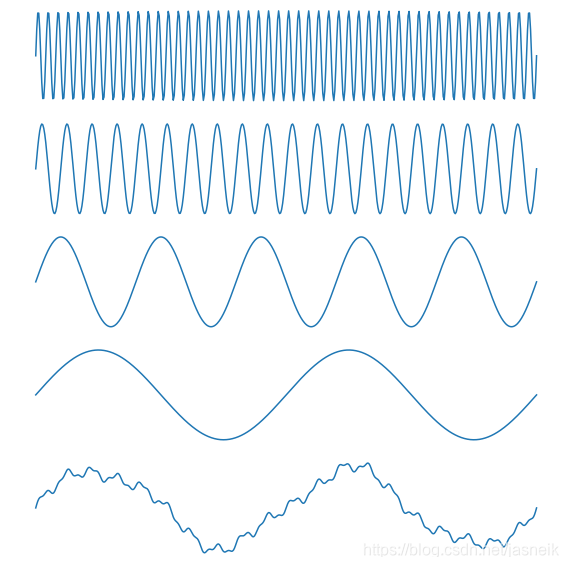
# 不同頻率的疊加
x = np.linspace(0, 1, 500)t = 50
A = 1
y_1 = A * np.sin(t * 2 * np.pi * x)t = 20
A = 2.5
y_2 = A * np.sin(t * 2 * np.pi * x)t = 5
A = 3
y_3 = A * np.sin(t * 2 * np.pi * x)t = 2
A = 20
y_4 = A * np.sin(t * 2 * np.pi * x)y_5 = y_1 + y_2 + y_3 + y_4fig = plt.figure(figsize=(8, 8))ax_1 = fig.add_subplot(5, 1, 1)
plt.plot(x, y_1), plt.xticks([]), plt.yticks([])
set_spines_invisible(ax_1)ax_2 = fig.add_subplot(5, 1, 2)
plt.plot(x, y_2), plt.xticks([]), plt.yticks([])
set_spines_invisible(ax_2)ax_3 = fig.add_subplot(5, 1, 3)
plt.plot(x, y_3), plt.xticks([]), plt.yticks([])
set_spines_invisible(ax_3)ax_4 = fig.add_subplot(5, 1, 4)
plt.plot(x, y_4), plt.xticks([]), plt.yticks([])
set_spines_invisible(ax_4)ax_5 = fig.add_subplot(5, 1, 5)
plt.plot(x, y_5), plt.xticks([]), plt.yticks([])
set_spines_invisible(ax_5)plt.tight_layout()
plt.show()