faster rcnn學習之rpn訓練全過程

上篇我們講解了rpn與fast rcnn的數據準備階段，接下來我們講解rpn的整個訓練過程。最后講解rpn訓練完畢后rpn的生成。

我們順著stage1_rpn_train.pt的內容講解。

name: "VGG_CNN_M_1024"
layer {name: 'input-data'type: 'Python'top: 'data'top: 'im_info'top: 'gt_boxes'python_param {module: 'roi_data_layer.layer'layer: 'RoIDataLayer'param_str: "'num_classes': 21"}
}
layer {name: "conv1"type: "Convolution"bottom: "data"top: "conv1"param { lr_mult: 0 decay_mult: 0 }param { lr_mult: 0 decay_mult: 0 }convolution_param {num_output: 96kernel_size: 7 stride: 2}
}
layer {name: "relu1"type: "ReLU"bottom: "conv1"top: "conv1"
}
layer {name: "norm1"type: "LRN"bottom: "conv1"top: "norm1"lrn_param {local_size: 5alpha: 0.0005beta: 0.75k: 2}
}
layer {name: "pool1"type: "Pooling"bottom: "norm1"top: "pool1"pooling_param {pool: MAXkernel_size: 3 stride: 2}
}
layer {name: "conv2"type: "Convolution"bottom: "pool1"top: "conv2"param { lr_mult: 1 }param { lr_mult: 2 }convolution_param {num_output: 256pad: 1 kernel_size: 5 stride: 2}
}
layer {name: "relu2"type: "ReLU"bottom: "conv2"top: "conv2"
}
layer {name: "norm2"type: "LRN"bottom: "conv2"top: "norm2"lrn_param {local_size: 5alpha: 0.0005beta: 0.75k: 2}
}
layer {name: "pool2"type: "Pooling"bottom: "norm2"top: "pool2"pooling_param {pool: MAXkernel_size: 3 stride: 2}
}
layer {name: "conv3"type: "Convolution"bottom: "pool2"top: "conv3"param { lr_mult: 1 }param { lr_mult: 2 }convolution_param {num_output: 512pad: 1 kernel_size: 3}
}
layer {name: "relu3"type: "ReLU"bottom: "conv3"top: "conv3"
}
layer {name: "conv4"type: "Convolution"bottom: "conv3"top: "conv4"param { lr_mult: 1 }param { lr_mult: 2 }convolution_param {num_output: 512pad: 1 kernel_size: 3}
}
layer {name: "relu4"type: "ReLU"bottom: "conv4"top: "conv4"
}
layer {name: "conv5"type: "Convolution"bottom: "conv4"top: "conv5"param { lr_mult: 1 }param { lr_mult: 2 }convolution_param {num_output: 512pad: 1 kernel_size: 3}
}
layer {name: "relu5"type: "ReLU"bottom: "conv5"top: "conv5"
}#========= RPN ============layer {name: "rpn_conv/3x3"type: "Convolution"bottom: "conv5"top: "rpn/output"param { lr_mult: 1.0 }param { lr_mult: 2.0 }convolution_param {num_output: 256kernel_size: 3 pad: 1 stride: 1weight_filler { type: "gaussian" std: 0.01 }bias_filler { type: "constant" value: 0 }}
}
layer {name: "rpn_relu/3x3"type: "ReLU"bottom: "rpn/output"top: "rpn/output"
}
layer {name: "rpn_cls_score"type: "Convolution"bottom: "rpn/output"top: "rpn_cls_score"param { lr_mult: 1.0 }param { lr_mult: 2.0 }convolution_param {num_output: 18   # 2(bg/fg) * 9(anchors)kernel_size: 1 pad: 0 stride: 1weight_filler { type: "gaussian" std: 0.01 }bias_filler { type: "constant" value: 0 }}
}
layer {name: "rpn_bbox_pred"type: "Convolution"bottom: "rpn/output"top: "rpn_bbox_pred"param { lr_mult: 1.0 }param { lr_mult: 2.0 }convolution_param {num_output: 36   # 4 * 9(anchors)kernel_size: 1 pad: 0 stride: 1weight_filler { type: "gaussian" std: 0.01 }bias_filler { type: "constant" value: 0 }}
}
layer {bottom: "rpn_cls_score"top: "rpn_cls_score_reshape"name: "rpn_cls_score_reshape"type: "Reshape"reshape_param { shape { dim: 0 dim: 2 dim: -1 dim: 0 } }
}
layer {name: 'rpn-data'type: 'Python'bottom: 'rpn_cls_score'bottom: 'gt_boxes'bottom: 'im_info'bottom: 'data'top: 'rpn_labels'top: 'rpn_bbox_targets'top: 'rpn_bbox_inside_weights'top: 'rpn_bbox_outside_weights'python_param {module: 'rpn.anchor_target_layer'layer: 'AnchorTargetLayer'param_str: "'feat_stride': 16"}
}
layer {name: "rpn_loss_cls"type: "SoftmaxWithLoss"bottom: "rpn_cls_score_reshape"bottom: "rpn_labels"propagate_down: 1propagate_down: 0top: "rpn_cls_loss"loss_weight: 1loss_param {ignore_label: -1normalize: true}
}
layer {name: "rpn_loss_bbox"type: "SmoothL1Loss"bottom: "rpn_bbox_pred"bottom: "rpn_bbox_targets"bottom: 'rpn_bbox_inside_weights'bottom: 'rpn_bbox_outside_weights'top: "rpn_loss_bbox"loss_weight: 1smooth_l1_loss_param { sigma: 3.0 }
}#========= RCNN ============layer {name: "dummy_roi_pool_conv5"type: "DummyData"top: "dummy_roi_pool_conv5"dummy_data_param {shape { dim: 1 dim: 18432 }data_filler { type: "gaussian" std: 0.01 }}
}
layer {name: "fc6"type: "InnerProduct"bottom: "dummy_roi_pool_conv5"top: "fc6"param { lr_mult: 0 decay_mult: 0 }param { lr_mult: 0 decay_mult: 0 }inner_product_param {num_output: 4096}
}
layer {name: "fc7"type: "InnerProduct"bottom: "fc6"top: "fc7"param { lr_mult: 0 decay_mult: 0 }param { lr_mult: 0 decay_mult: 0 }inner_product_param {num_output: 1024}
}
layer {name: "silence_fc7"type: "Silence"bottom: "fc7"
}

它的示意圖如下：這里借用了 http://blog.csdn.net/zy1034092330/article/details/62044941里的圖。

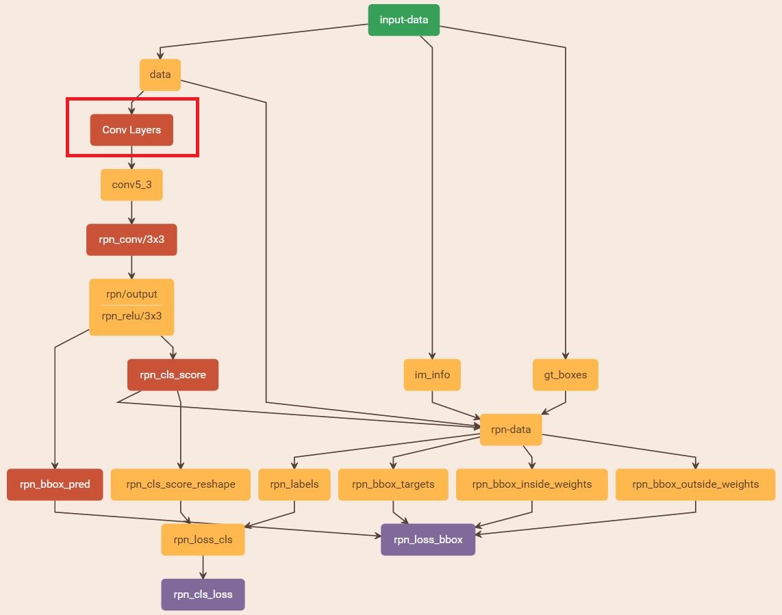
上面Conv layers包含了五層卷積層。接下來，對于第五層卷積層，進行了3*3的卷積操作，輸出了256個通道，當然大小與卷積前的大小相同。

然后開始分別接入了cls層與regression層。對于cls層，使用1*1的卷積操作輸出了18（9*2 bg/fg）個通道的feature map,大小不變。而對于regression層，也使用1*1的卷積層輸出了36(4*9)個通道的feature map，大小不變。?

對于cls層后又接了一個reshape層，為什么要接這個層呢？引用參考文獻[1]的話，其實只是為了便于softmax分類，至于具體原因這就要從caffe的實現形式說起了。在caffe基本數據結構blob中以如下形式保存數據：
blob=[batch_size, channel，height，width]
對應至上面的保存bg/fg anchors的矩陣，其在caffe blob中的存儲形式為[1, 2*9, H, W]。而在softmax分類時需要進行fg/bg二分類，所以reshape layer會將其變為[1, 2, 9*H, W]大小，即單獨“騰空”出來一個維度以便softmax分類，之后再reshape回復原狀。

我們可以用python模擬一下，看如下的程序：

>>> a=np.array([[[1,2],[3,4]],[[5,6],[7,8]],[[9,10],[11,12]],[[13,14],[15,16]]])

>>> a
array([[[ 1,  2],[ 3,  4]],[[ 5,  6],[ 7,  8]],[[ 9, 10],[11, 12]],[[13, 14],[15, 16]]])
>>> a.shape
(4L, 2L, 2L)

然后由于caffe中是行優先，numpy也如此，那么reshape一下的結果如下：

>>> b=a.reshape(2,4,2)
>>> b
array([[[ 1,  2],[ 3,  4],[ 5,  6],[ 7,  8]],[[ 9, 10],[11, 12],[13, 14],[15, 16]]])

從上面可以看出reshape是把相鄰通道的矩陣移到它的下面了。這樣就剩下兩個大的矩陣了，就可以相鄰通道之間進行softmax了。 從中其實我們也能發現，對于rpn每個點的18個輸出通道，前9個為背景的預測分數，而后9個為前景的預測分數。

假定softmax昨晚后，我們看看是否能夠回到原先？

>>> b.reshape(4,2,2)
array([[[ 1,  2],[ 3,  4]],[[ 5,  6],[ 7,  8]],[[ 9, 10],[11, 12]],[[13, 14],[15, 16]]])

果然又回到了原始的狀態。

而對于regression呢，不需要這樣的操作，那么他的36個通道是不是也是如上面18個通道那樣呢？即第一個9通道為dx,第二個為dy,第三個為dw，第五個是dh。還是我們比較容易想到的那種,即第一個通道是第一個盒子的回歸量(dx1,dy1,dw1,dh1),第二個為(dx2,dy2,dw,2,dh2).....。待后面查看對應的bbox_targets就知道了。先留個坑。

正如圖上所示，我們還需要準備一個層rpn-data。

layer {name: 'rpn-data'type: 'Python'bottom: 'rpn_cls_score'bottom: 'gt_boxes'bottom: 'im_info'bottom: 'data'top: 'rpn_labels'top: 'rpn_bbox_targets'top: 'rpn_bbox_inside_weights'top: 'rpn_bbox_outside_weights'python_param {module: 'rpn.anchor_target_layer'layer: 'AnchorTargetLayer'param_str: "'feat_stride': 16"}
}

這一層輸入四個量：data,gt_boxes,im_info,rpn_cls_score,其中前三個是我們在前面說過的，

data: ? ? ? ? 1*3*600*1000
gt_boxes: N*5, ? ? ? ? ? ? ? ? ? N為groundtruth box的個數，每一行為(x1, y1, x2, y2, cls) ，而且這里的gt_box是經過縮放的。
im_info： 1*3 ? ? ? ? ? ? ? ? ? （h,w,scale）

rpn_cls_score是cls層輸出的18通道，shape可以看成是1*18*H*W. ?

輸出為4個量：rpn_labels 、rpn_bbox_targets（回歸目標）、rpn_bbox_inside_weights（內權重）、rpn_bbox_outside_weights（外權重）。

通俗地來講，這一層產生了具體的anchor坐標，并與groundtruth box進行了重疊度計算，輸出了kabel與回歸目標。

接下來我們來看一下文件anchor_target_layer.py?

 def setup(self, bottom, top):layer_params = yaml.load(self.param_str_)    #在第5個卷積層后的feature map上的每個點取anchor,尺度為（8,16,32），結合后面的feat_stride為16，#再縮放回原來的圖像大小，正好尺度是(128,256,512),與paper一樣。anchor_scales = layer_params.get('scales', (8, 16, 32))  self._anchors = generate_anchors(scales=np.array(anchor_scales))  #產生feature map最左上角的那個點對應的anchor（x1,y1,x2,y2），# 尺度為原始圖像的尺度（可以看成是Im_info的寬和高尺度，或者是600*1000）。self._num_anchors = self._anchors.shape[0]   #9self._feat_stride = layer_params['feat_stride'] #16if DEBUG:print 'anchors:'print self._anchorsprint 'anchor shapes:'print np.hstack((  # 輸出寬和高self._anchors[:, 2::4] - self._anchors[:, 0::4], #第2列減去第0列self._anchors[:, 3::4] - self._anchors[:, 1::4], #第3列減去第1列))self._counts = cfg.EPSself._sums = np.zeros((1, 4))self._squared_sums = np.zeros((1, 4))self._fg_sum = 0self._bg_sum = 0self._count = 0# allow boxes to sit over the edge by a small amount  self._allowed_border = layer_params.get('allowed_border', 0)    height, width = bottom[0].data.shape[-2:]   #cls后的feature map的大小if DEBUG:print 'AnchorTargetLayer: height', height, 'width', widthA = self._num_anchors   # labelstop[0].reshape(1, 1, A * height, width)     # 顯然與rpn_cls_score_reshape保持相同的shape.# bbox_targetstop[1].reshape(1, A * 4, height, width)     # bbox_inside_weightstop[2].reshape(1, A * 4, height, width)# bbox_outside_weightstop[3].reshape(1, A * 4, height, width)

setup設置了top輸出的shape,并且做了一些準備工作。

接下來看forward函數。

 def forward(self, bottom, top):# Algorithm:## for each (H, W) location i#   generate 9 anchor boxes centered on cell i#   apply predicted bbox deltas at cell i to each of the 9 anchors# filter out-of-image anchors# measure GT overlapassert bottom[0].data.shape[0] == 1, \'Only single item batches are supported'     # 僅僅支持一張圖片# map of shape (..., H, W)height, width = bottom[0].data.shape[-2:]        # GT boxes (x1, y1, x2, y2, label)gt_boxes = bottom[1].data                          # im_infoim_info = bottom[2].data[0, :]if DEBUG:print ''print 'im_size: ({}, {})'.format(im_info[0], im_info[1])print 'scale: {}'.format(im_info[2])print 'height, width: ({}, {})'.format(height, width)print 'rpn: gt_boxes.shape', gt_boxes.shapeprint 'rpn: gt_boxes', gt_boxes# 1. Generate proposals from bbox deltas and shifted anchorsshift_x = np.arange(0, width) * self._feat_stride  shift_y = np.arange(0, height) * self._feat_stride shift_x, shift_y = np.meshgrid(shift_x, shift_y)shifts = np.vstack((shift_x.ravel(), shift_y.ravel(),shift_x.ravel(), shift_y.ravel())).transpose()# add A anchors (1, A, 4) to# cell K shifts (K, 1, 4) to get# shift anchors (K, A, 4)# reshape to (K*A, 4) shifted anchorsA = self._num_anchorsK = shifts.shape[0]all_anchors = (self._anchors.reshape((1, A, 4)) +shifts.reshape((1, K, 4)).transpose((1, 0, 2)))all_anchors = all_anchors.reshape((K * A, 4))total_anchors = int(K * A)                       # 根據左上角的anchor生成所有的anchor，這里將所有的anchor按照行排列。行：K*A(K= height*width ,A=9),列：4，且按照feature map按行優先這樣排下來。# only keep anchors inside the image   #取所有在圖像內部的anchorinds_inside = np.where((all_anchors[:, 0] >= -self._allowed_border) &(all_anchors[:, 1] >= -self._allowed_border) &(all_anchors[:, 2] < im_info[1] + self._allowed_border) &  # width(all_anchors[:, 3] < im_info[0] + self._allowed_border)    # height)[0]                                   if DEBUG:print 'total_anchors', total_anchorsprint 'inds_inside', len(inds_inside)# keep only inside anchorsanchors = all_anchors[inds_inside, :]if DEBUG:print 'anchors.shape', anchors.shape# label: 1 is positive, 0 is negative, -1 is dont carelabels = np.empty((len(inds_inside), ), dtype=np.float32)labels.fill(-1)# overlaps between the anchors and the gt boxes# overlaps (ex, gt)overlaps = bbox_overlaps(np.ascontiguousarray(anchors, dtype=np.float),np.ascontiguousarray(gt_boxes, dtype=np.float))argmax_overlaps = overlaps.argmax(axis=1)   #對于每一個anchor，取其重疊度最大的ground truth的序號max_overlaps = overlaps[np.arange(len(inds_inside)), argmax_overlaps]   #生成max_overlaps,(為一列)即每個anchor對應的最大重疊度gt_argmax_overlaps = overlaps.argmax(axis=0)          #對于每個類，選擇其對應的最大重疊度的anchor序號gt_max_overlaps = overlaps[gt_argmax_overlaps,       np.arange(overlaps.shape[1])]  #生成gt_max_overlaps，（為一行）即每類對應的最大重疊度gt_argmax_overlaps = np.where(overlaps == gt_max_overlaps)[0]  #找到那些等于gt_max_overlaps的anchor,這些anchor將參與訓練rpn# 找到所有overlaps中所有等于gt_max_overlaps的元素，因為gt_max_overlaps對于每個非負類別只保留一個# anchor，如果同一列有多個相等的最大IOU overlap值，那么就需要把其他的幾個值找到，并在后面將它們# 的label設為1，即認為它們是object，畢竟在RPN的cls任務中，只要認為它是否是個object即可，即一個# 二分類問題。   (總結)# 如下設置了前景(1)、背景(0)以及不關心(-1)的anchor標簽if not cfg.TRAIN.RPN_CLOBBER_POSITIVES:# assign bg labels first so that positive labels can clobber themlabels[max_overlaps < cfg.TRAIN.RPN_NEGATIVE_OVERLAP] = 0    #對于最大重疊度低于0.3的設為背景# fg label: for each gt, anchor with highest overlap  labels[gt_argmax_overlaps] = 1   # fg label: above threshold IOUlabels[max_overlaps >= cfg.TRAIN.RPN_POSITIVE_OVERLAP] = 1 if cfg.TRAIN.RPN_CLOBBER_POSITIVES:# assign bg labels last so that negative labels can clobber positiveslabels[max_overlaps < cfg.TRAIN.RPN_NEGATIVE_OVERLAP] = 0# 取前景與背景的anchor各一半，目前一批有256個anchor.# subsample positive labels if we have too manynum_fg = int(cfg.TRAIN.RPN_FG_FRACTION * cfg.TRAIN.RPN_BATCHSIZE)   #256*0.5=128fg_inds = np.where(labels == 1)[0]if len(fg_inds) > num_fg:disable_inds = npr.choice(fg_inds, size=(len(fg_inds) - num_fg), replace=False)labels[disable_inds] = -1# subsample negative labels if we have too manynum_bg = cfg.TRAIN.RPN_BATCHSIZE - np.sum(labels == 1)  #另一半256*0.5=128bg_inds = np.where(labels == 0)[0]if len(bg_inds) > num_bg:disable_inds = npr.choice(bg_inds, size=(len(bg_inds) - num_bg), replace=False)labels[disable_inds] = -1#print "was %s inds, disabling %s, now %s inds" % (#len(bg_inds), len(disable_inds), np.sum(labels == 0))#計算了所有在內部的anchor與對應的ground truth的回歸量bbox_targets = np.zeros((len(inds_inside), 4), dtype=np.float32)bbox_targets = _compute_targets(anchors, gt_boxes[argmax_overlaps, :])#只有前景類內部權重才非0，參與回歸bbox_inside_weights = np.zeros((len(inds_inside), 4), dtype=np.float32)bbox_inside_weights[labels == 1, :] = np.array(cfg.TRAIN.RPN_BBOX_INSIDE_WEIGHTS) #(1.0, 1.0, 1.0, 1.0)# Give the positive RPN examples weight of p * 1 / {num positives}# and give negatives a weight of (1 - p)/(num negative)    # Set to -1.0 to use uniform example weightingbbox_outside_weights = np.zeros((len(inds_inside), 4), dtype=np.float32)if cfg.TRAIN.RPN_POSITIVE_WEIGHT < 0:# uniform weighting of examples (given non-uniform sampling)num_examples = np.sum(labels >= 0)positive_weights = np.ones((1, 4)) * 1.0 / num_examplesnegative_weights = np.ones((1, 4)) * 1.0 / num_exampleselse:assert ((cfg.TRAIN.RPN_POSITIVE_WEIGHT > 0) &(cfg.TRAIN.RPN_POSITIVE_WEIGHT < 1))positive_weights = (cfg.TRAIN.RPN_POSITIVE_WEIGHT /np.sum(labels == 1))negative_weights = ((1.0 - cfg.TRAIN.RPN_POSITIVE_WEIGHT) /np.sum(labels == 0))bbox_outside_weights[labels == 1, :] = positive_weights  # 前景與背景anchor的外參數相同，都是1/anchor個數bbox_outside_weights[labels == 0, :] = negative_weightsif DEBUG:self._sums += bbox_targets[labels == 1, :].sum(axis=0)self._squared_sums += (bbox_targets[labels == 1, :] ** 2).sum(axis=0)self._counts += np.sum(labels == 1)means = self._sums / self._countsstds = np.sqrt(self._squared_sums / self._counts - means ** 2)print 'means:'print meansprint 'stdevs:'print stds# map up to original set of anchors 生成全部anchor的數據，將非0的數據填入。labels = _unmap(labels, total_anchors, inds_inside, fill=-1)bbox_targets = _unmap(bbox_targets, total_anchors, inds_inside, fill=0)bbox_inside_weights = _unmap(bbox_inside_weights, total_anchors, inds_inside, fill=0)bbox_outside_weights = _unmap(bbox_outside_weights, total_anchors, inds_inside, fill=0)if DEBUG:print 'rpn: max max_overlap', np.max(max_overlaps)print 'rpn: num_positive', np.sum(labels == 1)print 'rpn: num_negative', np.sum(labels == 0)self._fg_sum += np.sum(labels == 1)self._bg_sum += np.sum(labels == 0)self._count += 1print 'rpn: num_positive avg', self._fg_sum / self._countprint 'rpn: num_negative avg', self._bg_sum / self._count# labels labels = labels.reshape((1, height, width, A)).transpose(0, 3, 1, 2)labels = labels.reshape((1, 1, A * height, width))top[0].reshape(*labels.shape)top[0].data[...] = labels# bbox_targetsbbox_targets = bbox_targets \.reshape((1, height, width, A * 4)).transpose(0, 3, 1, 2)top[1].reshape(*bbox_targets.shape)top[1].data[...] = bbox_targets# bbox_inside_weightsbbox_inside_weights = bbox_inside_weights \.reshape((1, height, width, A * 4)).transpose(0, 3, 1, 2)assert bbox_inside_weights.shape[2] == heightassert bbox_inside_weights.shape[3] == widthtop[2].reshape(*bbox_inside_weights.shape)top[2].data[...] = bbox_inside_weights# bbox_outside_weightsbbox_outside_weights = bbox_outside_weights \.reshape((1, height, width, A * 4)).transpose(0, 3, 1, 2)assert bbox_outside_weights.shape[2] == heightassert bbox_outside_weights.shape[3] == widthtop[3].reshape(*bbox_outside_weights.shape)top[3].data[...] = bbox_outside_weights

這里已經有詳細的注釋，總的來說，rpn_cls_score的作用就是告知第五層feature map的寬和高。便于決定生成多少個anchor. 而其他的bottom輸入才最終決定top的輸出。

首先這里生成了所有feature map各點對應的anchors。生成的方式很特別，先考慮了左上角一個點的anchor生成，考慮到feat_stride=16，所以這個點對應原始圖像（這里統一指縮放后image）的(0,0,15,15)感受野。然后取其中心點，生成比例為1:1,1:2,2:1，尺度在128,256,512的9個anchor.然后考慮使用平移生成其他的anchor.

然后過濾掉那些不在圖像內部的anchor. 對于剩下的anchor,計算與gt_boxes的重疊度，再分別計算label,bbox_targets,bbox_inside_weights,bbox_outside_weights.

最后將內部的anchor的相關變量擴充到所有的anchor,只不過不在內部的為0即可。尤其值得說的是對于內部的anchor,bbox_targets都進行了運算。但是選取了256個anchor,前景與背景比例為1:1，bbox_inside_weights中只有label=1,即前景才進行了設置。正如論文所說，對于回歸項，需要內部參數來約束，bbox_inside_weights正好起到了這個作用。

我們統計一下top的shape:

rpn_labels ： (1, 1, 9 * height, width)

rpn_bbox_targets（回歸目標）： (1, 36，height, width)

rpn_bbox_inside_weights（內權重）：(1, 36，height, width)

rpn_bbox_outside_weights（外權重）：(1, 36，height, width)

回到stage1_rpn_train.pt，接下里我們就可以利用rpn_cls_score_reshape與rpn_labels計算SoftmaxWithLoss，輸出rpn_cls_loss。

而regression可以利用rpn_bbox_pred，rpn_bbox_targets，rpn_bbox_inside_weights，rpn_bbox_outside_weights計算SmoothL1Loss，輸出rpn_loss_bbox。

回到我們之前有一個問題rpn_bbox_pred的shape怎么構造的。其實從rpn_bbox_targets的生成過程中可以推斷出應該采用后一種，即第一個盒子的回歸量(dx1,dy1,dw1,dh1),第二個為(dx2,dy2,dw,2,dh2).....，這樣順序著來。

其實怎么樣認為都是從我們方便的角度出發。

至此我們完成了rpn的前向過程，反向過程中只需注意AnchorTargetLayer不參與反向傳播。因為它提供的都是源數據。

參考：

1. ?http://blog.csdn.net/zy1034092330/article/details/62044941?