參考文獻：

https://zhuanlan.zhihu.com/p/71328244

目錄

1.可視化計算圖

2.可視化參數

3. 遠程tensorboard

4、報錯

---

真是出來混遲早是要還的，之前一直拒絕學習Tensorboard，因為實在是有替代方案，直到發現到了不得不用的地步。下面主要介紹一下怎么使用Tensorboard來可視化參數，損失以及準確率等變量。

1.可視化計算圖

下面是一個單層網絡的手寫體分類示例：

import tensorflow as tf
from tensorflow.examples.tutorials.mnist import input_datamnist = input_data.read_data_sets("MNIST_data", one_hot=True)batch_size = 100
n_batch = mnist.train.num_examples // batch_sizewith tf.name_scope('input'):x = tf.placeholder(dtype=tf.float32, shape=[None, 784], name='x_input')y = tf.placeholder(dtype=tf.int32, shape=[None, 10], name='y_input')with tf.name_scope('layer'):with tf.name_scope('weights'):W = tf.Variable(tf.random_uniform([784, 10]), name='w')with tf.name_scope('biases'):b = tf.Variable(tf.zeros(shape=[10], dtype=tf.float32), name='b')with tf.name_scope('softmax'):prediction = tf.nn.softmax(tf.nn.xw_plus_b(x, W, b))
with tf.name_scope('Loss'):loss = tf.reduce_mean(tf.nn.softmax_cross_entropy_with_logits(labels=y, logits=prediction))
with tf.name_scope('train'):train_step = tf.train.GradientDescentOptimizer(0.01).minimize(loss)
with tf.name_scope('acc'):correct_prediction = tf.equal(tf.argmax(y, 1), tf.argmax(prediction, 1))acc = tf.reduce_mean(tf.cast(correct_prediction, tf.float32))with tf.Session() as sess:sess.run(tf.global_variables_initializer())writer = tf.summary.FileWriter('logs/', sess.graph)for epoch in range(20):for batch in range(n_batch):batch_x, batch_y = mnist.train.next_batch(batch_size)_, accuracy = sess.run([train_step, acc], feed_dict={x: batch_x, y: batch_y})if batch % 50 == 0:print("### Epoch: {}, batch: {} acc on train: {}".format(epoch, batch, accuracy))accuracy = sess.run(acc, feed_dict={x: mnist.test.images, y: mnist.test.labels})print("### Epoch: {},  acc on test: {}".format(epoch, accuracy))

其計算圖的可視化結果如下所示：

?

?

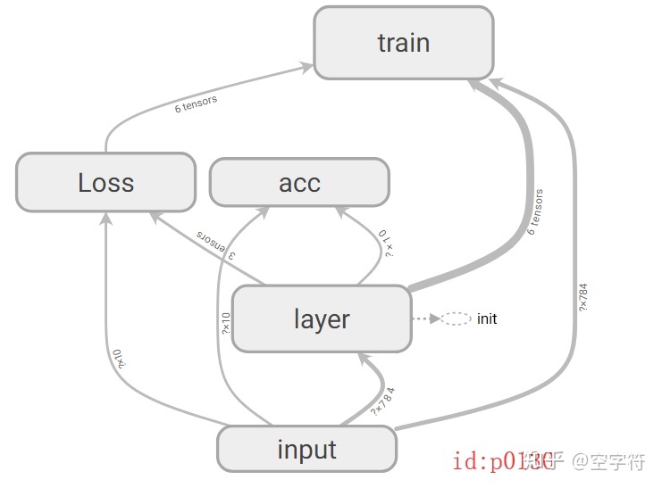
其中圖中灰色的圓角矩形就是代碼中的一個個命名空間tf.name_scope()，而且命名空間是可以嵌套定義的。從計算圖中，可以清楚的看到各個操作的詳細信息，以及數據量的形狀和流向等。這一操作的實現，就全靠第31行代碼。執行完這句代碼后，會在你指定路徑（此處為代碼所在路徑的logs文件夾中）中生成一個類似名為events.out.tfevents.1561711787的文件。其打開步驟如下：

• 首先需要安裝tensorflow和tensorboard；
• 打開命令行（Linux終端)，進入到log的上一層目錄；
• 運行命令tensorboard --logdir=logs
• 如果成功，則會有以下提示：
  • TensorBoard 1.5.1 at http://DESKTOP-70LJI62:6006 (Press CTRL+C to quit)
  
  
• 如果有任何報錯，最直接的辦法就是卸載tensorflow重新安裝，若是有多個環境建議用Anaconda管理
• 將后面的地址粘貼到瀏覽器中（最好是谷歌），然后就能看到了，可以雙擊各個結點查看詳細信息

2.可視化參數

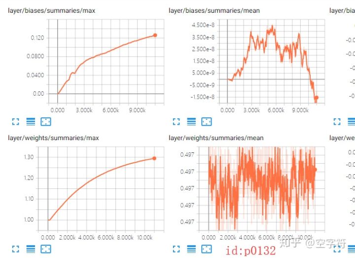
可視化網絡計算圖不是太有意義，而更有意義的是在訓練網絡的同時能夠看到一些參數的變換曲線圖（如：準確率，損失等），以便于更好的分析網絡。

?

?

要實現這個操作，只需要添加對應的tf.summary.scalar('acc', acc)語句即可，然后最后合并所有的summary即可。但是，通常情況下網絡層的參數都不是標量，而是矩陣這類的；對于這種變量，通常的做法就是計算其最大、最小、平均值以及直方圖等。由于對于很多參數都會用到同樣的這幾個操作，所以在這里就統一定義函數：

def variable_summaries(var):with tf.name_scope('summaries'):mean = tf.reduce_mean(var)tf.summary.scalar('mean', mean)with tf.name_scope('stddev'):stddev = tf.sqrt(tf.reduce_mean(tf.square(var - mean)))tf.summary.scalar('stddev', stddev)tf.summary.scalar('max', tf.reduce_max(var))tf.summary.scalar('min', tf.reduce_min(var))tf.summary.histogram('histogram', var)

然后在需要可視化參數的地方，調用這個函數即可。

mnist = input_data.read_data_sets("MNIST_data", one_hot=True)batch_size = 100n_batch = mnist.train.num_examples // batch_size
with tf.name_scope('input'):x = tf.placeholder(dtype=tf.float32, shape=[None, 784], name='x_input')y = tf.placeholder(dtype=tf.int32, shape=[None, 10], name='y_input')with tf.name_scope('layer'):with tf.name_scope('weights'):W = tf.Variable(tf.random_uniform([784, 10]), name='w')variable_summaries(W)####with tf.name_scope('biases'):b = tf.Variable(tf.zeros(shape=[10], dtype=tf.float32), name='b')variable_summaries(b)with tf.name_scope('softmax'):prediction = tf.nn.softmax(tf.nn.xw_plus_b(x, W, b))
with tf.name_scope('Loss'):loss = tf.reduce_mean(tf.nn.softmax_cross_entropy_with_logits(labels=y, logits=prediction))tf.summary.scalar('loss', loss)
with tf.name_scope('train'):train_step = tf.train.GradientDescentOptimizer(0.01).minimize(loss)
with tf.name_scope('acc'):correct_prediction = tf.equal(tf.argmax(y, 1), tf.argmax(prediction, 1))acc = tf.reduce_mean(tf.cast(correct_prediction, tf.float32))tf.summary.scalar('acc', acc)merged = tf.summary.merge_all()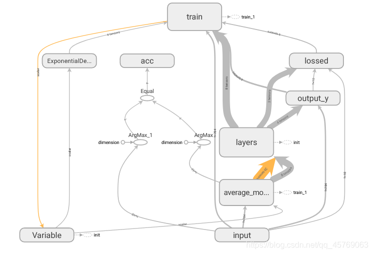
with tf.Session() as sess:sess.run(tf.global_variables_initializer())writer = tf.summary.FileWriter('logs/', sess.graph)for epoch in range(20):for batch in range(n_batch):batch_x, batch_y = mnist.train.next_batch(batch_size)_, summary, accuracy = sess.run([train_step, merged, acc], feed_dict={x: batch_x, y: batch_y})if batch % 50 == 0:print("### Epoch: {}, batch: {} acc on train: {}".format(epoch, batch, accuracy))writer.add_summary(summary, epoch * n_batch + batch)accuracy = sess.run(acc, feed_dict={x: mnist.test.images, y: mnist.test.labels})print("### Epoch: {},  acc on test: {}".format(epoch, accuracy))

如上代碼中的第14、17、22、28行所示。最后，在每次迭代的時候，將合并后的merged進行計算并寫道本地文件中（第40行）。最后，按照上面的方法，用tensorboard打開即可。

注：這個不用等到整個過程訓練完才能可視化，而是你在訓練過程中就能看到的，而且是每30秒根據生成的數據刷新一次，還是很Nice的。

?

?

3. 遠程tensorboard

由于條件所限，通常在進行深度學習時都是在遠處的服務器上進行訓練的，所以此時該怎么在本地電腦可視化呢？答案是利用SSH的方向隧道技術，將服務器上的端口數據轉發到本地對應的端口，然后就能在本地方法服務器上的日志數據了。

從上面連接成功后的提示可以知道，tensorboard所用到的端口時6006（沒準兒哪天就換了），所以我們只需將該端口的數據轉發到本地即可。

• ssh -L 16006:127.0.0.1:6006 account@server.address
• 其中16006是本地的任意端口，只要不和本地應用有沖突就行，隨便寫；
• 后面的account指你服務器的用戶名，緊接是Ip

windows的話，直接在命令行里執行這條令就行（也不知道啥時候windows命令行也支持ssh了）

在登陸成功后（此時已遠程登陸了服務器），同樣進入到logs目錄的上層目錄，然后運行tensorboard --logdir=logs；最后，在本地瀏覽器中運行127.0.0.1:16006即可。

?

4、報錯

可能會出“AttributeError: module 'tensorflow' has no attribute 'io'”錯誤

這可能是因為tensorboard版本過高或者和tensorflow版本不匹配導致

本人tensorflow版本為1.5.0，tensorboard版本為1.8.0,最終解決了報錯