01、Tensorflow實現二元手寫數字識別（二分類問題）

開始學習機器學習啦，已經把吳恩達的課全部刷完了，現在開始熟悉一下復現代碼。對這個手寫數字實部比較感興趣，作為入門的素材非常合適。

基于Tensorflow 2.10.0

1、識別目標

識別手寫僅僅是為了區分手寫的0和1，所以實際上是一個二分類問題。

2、Tensorflow算法實現

STEP1：導入相關包

import numpy as np
import tensorflow as tf
from keras.models import Sequential
from keras.layers import Dense
from sklearn.model_selection import train_test_split
import matplotlib.pyplot as plt
import warnings
import logging
from sklearn.metrics import accuracy_score

import numpy as np:這是引入numpy庫，并為其設置一個縮寫np。Numpy是Python中用于大規模數值計算的庫，它提供了多維數組對象及一系列操作這些數組的函數。

import tensorflow as tf:這是引入tensorflow庫，并為其設置一個縮寫tf。TensorFlow是一個開源的深度學習框架，它被廣泛用于各種深度學習應用。

from keras.models import Sequential:這是從Keras庫中引入Sequential模型。Keras是一個高級神經網絡API，它可以運行在TensorFlow之上。Sequential模型是Keras中的線性堆棧模型，允許你簡單地堆疊多個網絡層。

from keras.layers import Dense:這是從Keras庫中引入Dense層。Dense層是神經網絡中的全連接層，每個輸入節點與輸出節點都是連接的。

from sklearn.model_selection import train_test_split:這是從scikit-learn庫中引入train_test_split函數。這個函數用于將數據分割為訓練集和測試集。

import matplotlib.pyplot as plt:這是引入matplotlib的pyplot模塊，并為其設置一個縮寫plt。Matplotlib是Python中的繪圖庫，而pyplot是其中的一個模塊，用于繪制各種圖形和圖像。

import warnings:這是引入Python的標準警告庫，它可以用來發出警告，或者過濾掉不需要的警告。

import logging:這是引入Python的標準日志庫，用于記錄日志信息，方便追蹤和調試代碼。

from sklearn.metrics import accuracy_score:這是從scikit-learn庫中引入accuracy_score函數。這個函數用于計算分類準確率，常用于評估分類模型的性能。

---

STEP2:屏蔽無用警告并允許中文

logging.getLogger("tensorflow").setLevel(logging.ERROR)
tf.autograph.set_verbosity(0)
warnings.simplefilter(action='ignore', category=FutureWarning)
# 支持中文顯示
plt.rcParams['font.sans-serif']=['SimHei']
plt.rcParams['axes.unicode_minus']=False

logging.getLogger(“tensorflow”).setLevel(logging.ERROR)：這行代碼用于設置 TensorFlow 的日志級別為 ERROR。這意味著只有當 TensorFlow 中發生錯誤時，才會在日志中輸出相關信息。較低級別的日志信息（如 WARNING、INFO、DEBUG）將被忽略。

tf.autograph.set_verbosity(0)：這行代碼用于設置 TensorFlow 的自動圖形（Autograph）日志的冗長級別為 0。這意味著在將 Python 代碼轉換為 TensorFlow 圖形代碼時，將不會輸出任何日志信息。這有助于減少日志噪音，使日志更加干凈。

warnings.simplefilter(action=‘ignore’,category=FutureWarning)：這行代碼用于忽略所有 FutureWarning 類型的警告。在 Python中，當使用某些即將過時或未來版本中可能發生變化的特性時，通常會發出 FutureWarning。通過設置action=‘ignore’，代碼將不會輸出這類警告，使控制臺輸出更加干凈。

plt.rcParams[‘font.sans-serif’]=[‘SimHei’]：這行代碼用于設置 matplotlib 中的默認無襯線字體為 SimHei。SimHei 是一種常用于顯示中文的字體，這樣設置后，matplotlib 將在繪圖時使用 SimHei 字體來顯示中文，從而避免中文亂碼問題。

plt.rcParams[‘axes.unicode_minus’]=False：這行代碼用于解決 matplotlib
中負號顯示異常的問題。默認情況下，matplotlib 可能無法正確顯示負號，將其設置為 False 可以使用 ASCII字符作為負號，從而正常顯示。

---

STEP3:導入并劃分數據集

劃分10%作為測試：

X, y = load_data()
print('The shape of X is: ' + str(X.shape))
print('The shape of y is: ' + str(y.shape))
X_train, X_test, y_train, y_test = train_test_split(X, y, test_size=0.1, random_state=42)

---

STEP4:模型構建與訓練

# 構建模型，三層模型進行分類，第一層輸入100個神經元...
model = Sequential([tf.keras.Input(shape=(400,)),    #specify input size### START CODE HERE ###Dense(100, activation='sigmoid'),Dense(10, activation='sigmoid'),Dense(1, activation='sigmoid')### END CODE HERE ###], name = "my_model"
)
# 打印三層模型的參數
model.summary()
# 模型設定，學習率0.001，因為是分類，使用BinaryCrossentropy損失函數
model.compile(loss=tf.keras.losses.BinaryCrossentropy(),optimizer=tf.keras.optimizers.Adam(0.001),
)
# 開始訓練，訓練循環20
model.fit(X_train,y_train,epochs=20
)

---

STEP5:結果可視化與打印準確度信息
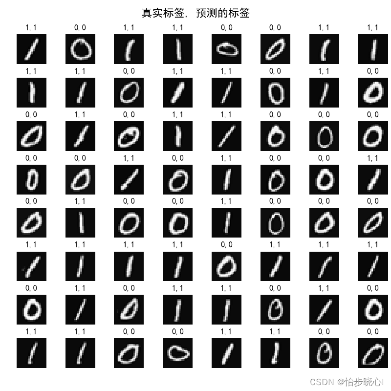
原始的輸入的數據集是400 * 1000的數組，共包含1000個手寫數字的數據，其中400為20*20像素的圖片，因此對每個400的數組進行reshape((20, 20))可以得到原始的圖片進而繪圖。

# 繪制測試集的預測結果，繪制64個
fig, axes = plt.subplots(8, 8, figsize=(8, 8))
fig.tight_layout(pad=0.1, rect=[0, 0.03, 1, 0.92])  # [left, bottom, right, top]
for i, ax in enumerate(axes.flat):# Select random indicesrandom_index = np.random.randint(X_test.shape[0])# Select rows corresponding to the random indices and# reshape the imageX_random_reshaped = X_test[random_index].reshape((20, 20)).T# Display the imageax.imshow(X_random_reshaped, cmap='gray')# Predict using the Neural Networkprediction = model.predict(X_test[random_index].reshape(1, 400))if prediction >= 0.5:yhat = 1else:yhat = 0# Display the label above the imageax.set_title(f"{y_test[random_index, 0]},{yhat}")ax.set_axis_off()
fig.suptitle("真實標簽, 預測的標簽", fontsize=16)
plt.show()# 給出預測的測試集誤差
y_pred=model.predict(X_test)
print("測試數據集準確率為：", accuracy_score(y_test, np.round(y_pred)))

3、運行結果

按照最初的劃分，數據集包含1000個數據，劃分10%為測試集，也就是100個數據。結果可視化隨機選擇其中的64個數據繪圖，每個圖像的上方標明了其真實標簽和預測的結果，這個是一個非常簡單的示例，準確度還是非常高的。

4、工程下載與全部代碼

工程鏈接：Tensorflow實現二元手寫數字識別（二分類問題）

import numpy as np
import tensorflow as tf
from keras.models import Sequential
from keras.layers import Dense
from sklearn.model_selection import train_test_split
import matplotlib.pyplot as plt
import warnings
import logging
from sklearn.metrics import accuracy_scorelogging.getLogger("tensorflow").setLevel(logging.ERROR)
tf.autograph.set_verbosity(0)
warnings.simplefilter(action='ignore', category=FutureWarning)
# 支持中文顯示
plt.rcParams['font.sans-serif']=['SimHei']
plt.rcParams['axes.unicode_minus']=False# load dataset
def load_data():X = np.load("Handwritten_Digit_Recognition_data/X.npy")y = np.load("Handwritten_Digit_Recognition_data/y.npy")X = X[0:1000]y = y[0:1000]return X, y# 加載數據集，查看數據集大小，可以看到有1000個數據集，每個輸入是20*20=400大小的圖片
X, y = load_data()
print('The shape of X is: ' + str(X.shape))
print('The shape of y is: ' + str(y.shape))
X_train, X_test, y_train, y_test = train_test_split(X, y, test_size=0.1, random_state=42)# # 下面畫圖，隨便從原數據取出幾個畫圖，可以注釋
# m, n = X.shape
# fig, axes = plt.subplots(8, 8, figsize=(8, 8))
# fig.tight_layout(pad=0.1)
# for i, ax in enumerate(axes.flat):
#     # Select random indices
#     random_index = np.random.randint(m)
#     # Select rows corresponding to the random indices and
#     # 將1*400的數據轉換為20*20的圖像格式
#     X_random_reshaped = X[random_index].reshape((20, 20)).T
#     # Display the image
#     ax.imshow(X_random_reshaped, cmap='gray')
#     # Display the label above the image
#     ax.set_title(y[random_index, 0])
#     ax.set_axis_off()
# plt.show()# 構建模型，三層模型進行分類，第一層輸入25個神經元...
model = Sequential([tf.keras.Input(shape=(400,)),    #specify input size### START CODE HERE ###Dense(100, activation='sigmoid'),Dense(10, activation='sigmoid'),Dense(1, activation='sigmoid')### END CODE HERE ###], name = "my_model"
)
# 打印三層模型的參數
model.summary()
# 模型設定，學習率0.001，因為是分類，使用BinaryCrossentropy損失函數
model.compile(loss=tf.keras.losses.BinaryCrossentropy(),optimizer=tf.keras.optimizers.Adam(0.001),
)
# 開始訓練，訓練循環20
model.fit(X_train,y_train,epochs=20
)# 繪制測試集的預測結果，繪制64個
fig, axes = plt.subplots(8, 8, figsize=(8, 8))
fig.tight_layout(pad=0.1, rect=[0, 0.03, 1, 0.92])  # [left, bottom, right, top]
for i, ax in enumerate(axes.flat):# Select random indicesrandom_index = np.random.randint(X_test.shape[0])# Select rows corresponding to the random indices and# reshape the imageX_random_reshaped = X_test[random_index].reshape((20, 20)).T# Display the imageax.imshow(X_random_reshaped, cmap='gray')# Predict using the Neural Networkprediction = model.predict(X_test[random_index].reshape(1, 400))if prediction >= 0.5:yhat = 1else:yhat = 0# Display the label above the imageax.set_title(f"{y_test[random_index, 0]},{yhat}")ax.set_axis_off()
fig.suptitle("真實標簽, 預測的標簽", fontsize=16)
plt.show()# 給出預測的測試集誤差
y_pred=model.predict(X_test)
print("測試數據集準確率為：", accuracy_score(y_test, np.round(y_pred)))