模型匯總-數學建模

一、優化模型

1.線性規劃

線性規劃（Linear Programming, LP）是一種數學優化方法，用于在給定的線性約束條件下，找到線性目標函數的最大值或最小值。它是運籌學中最常用的方法之一。

線性規劃的標準形式

最大化問題標準形式：

maximize: c?x
subject to: Ax ≤ bx ≥ 0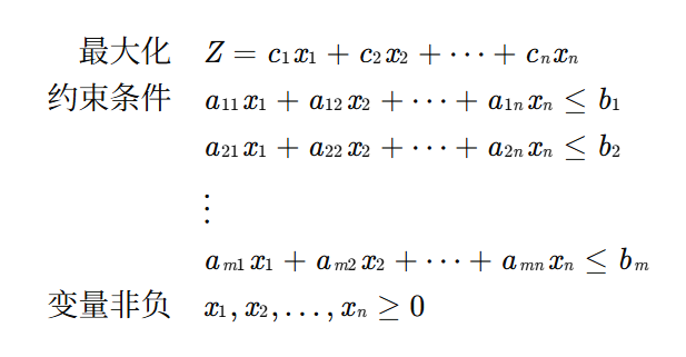

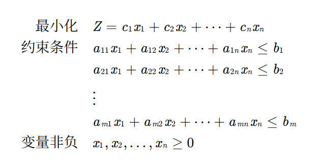
最小化問題標準形式：

minimize: c?x
subject to: Ax ≥ bx ≥ 0

其中：

x 是決策變量向量
c 是目標函數系數向量
A 是約束條件系數矩陣
b 是約束條件右側常數向量

Python實現線性規劃

我們將使用SciPy庫中的linprog函數來解決線性規劃問題。

安裝必要的庫

pip install scipy numpy matplotlib

簡單的最小化問題示例：

import numpy as np
from scipy.optimize import linprog
import matplotlib.pyplot as plt# 定義目標函數系數（注意：linprog默認求最小值，所以對于最大化問題需要取負）
c = [-1, 4]  # 原目標函數為 -x1 + 4x2，但linprog求最小值，所以這里系數不變# 定義不等式約束（左側系數矩陣）
A = [[1, -1],   # x1 - x2 ≤ 4[2, 1],    # 2x1 + x2 ≤ 14[1, 3]     # x1 + 3x2 ≤ 18
]# 定義不等式約束（右側常數向量）
b = [4, 14, 18]# 定義變量邊界
x_bounds = (0, None)  # x1 ≥ 0
y_bounds = (0, None)  # x2 ≥ 0# 求解線性規劃問題
result = linprog(c, A_ub=A, b_ub=b, bounds=[x_bounds, y_bounds], method='highs')# 輸出結果
print("優化結果:")
print(f"狀態: {result.message}")
print(f"最優解: x1 = {result.x[0]:.2f}, x2 = {result.x[1]:.2f}")
print(f"最優目標函數值: {result.fun:.2f}")
print(f"迭代次數: {result.nit}")# 可視化
def plot_feasible_region():# 創建網格x = np.linspace(0, 10, 400)y = np.linspace(0, 10, 400)X, Y = np.meshgrid(x, y)# 約束條件constraint1 = X - Y <= 4    # x1 - x2 ≤ 4constraint2 = 2*X + Y <= 14 # 2x1 + x2 ≤ 14constraint3 = X + 3*Y <= 18 # x1 + 3x2 ≤ 18non_negative = (X >= 0) & (Y >= 0)# 可行域feasible = constraint1 & constraint2 & constraint3 & non_negativeplt.figure(figsize=(10, 8))# 繪制可行域plt.imshow(feasible.astype(int), extent=(x.min(), x.max(), y.min(), y.max()), origin="lower", cmap="Greys", alpha=0.3)# 繪制約束線plt.plot(x, x - 4, label=r'$x_1 - x_2 = 4$')plt.plot(x, 14 - 2*x, label=r'$2x_1 + x_2 = 14$')plt.plot(x, (18 - x)/3, label=r'$x_1 + 3x_2 = 18$')# 繪制最優解點plt.plot(result.x[0], result.x[1], 'ro', markersize=10, label='最優解')# 繪制目標函數等值線Z = -X + 4*Y  # 目標函數值contours = plt.contour(X, Y, Z, levels=10, colors='gray', alpha=0.5)plt.clabel(contours, inline=True, fontsize=8)plt.xlim(0, 10)plt.ylim(0, 10)plt.xlabel(r'$x_1$')plt.ylabel(r'$x_2$')plt.title('線性規劃問題可視化')plt.legend()plt.grid(True)plt.show()plot_feasible_region()

示例2：生產計劃問題（最大化問題）

# 最大化問題：利潤 = 3A + 5B
# 由于linprog默認求最小值，我們需要對目標函數系數取負# 目標函數系數（取負是因為要求最大值）
c = [-3, -5]  # 最大化 3A + 5B 等價于最小化 -3A -5B# 約束條件系數矩陣
A = [[2, 1],   # 2A + B ≤ 10[1, 2]    # A + 2B ≤ 8
]# 約束條件右側常數
b = [10, 8]# 變量邊界
bounds = [(0, None), (0, None)]# 求解
result = linprog(c, A_ub=A, b_ub=b, bounds=bounds, method='highs')print("\n生產計劃問題結果:")
print(f"狀態: {result.message}")
print(f"最優生產計劃: 產品A = {result.x[0]:.2f}, 產品B = {result.x[1]:.2f}")
print(f"最大利潤: {-result.fun:.2f}元")  # 取負得到原始目標函數值

示例3：更復雜的線性規劃問題

# 最小化：-2x1 + x2 - x3
# 約束：
# x1 + x2 + x3 ≤ 6
# -x1 + 2x2 ≤ 4
# x1, x2, x3 ≥ 0c = [-2, 1, -1]  # 目標函數系數A = [[1, 1, 1],   # x1 + x2 + x3 ≤ 6[-1, 2, 0]   # -x1 + 2x2 ≤ 4
]b = [6, 4]bounds = [(0, None), (0, None), (0, None)]result = linprog(c, A_ub=A, b_ub=b, bounds=bounds, method='highs')print("\n復雜線性規劃問題結果:")
print(f"狀態: {result.message}")
print(f"最優解: x1 = {result.x[0]:.2f}, x2 = {result.x[1]:.2f}, x3 = {result.x[2]:.2f}")
print(f"最優目標函數值: {result.fun:.2f}")

處理等式約束

# 最小化：2x1 + 3x2
# 約束：
# x1 + x2 = 10
# 2x1 + x2 ≥ 15
# x1 ≥ 0, x2 ≥ 0c = [2, 3]  # 目標函數系數# 等式約束
A_eq = [[1, 1]]  # x1 + x2 = 10
b_eq = [10]# 不等式約束
A_ub = [[-2, -1]]  # 2x1 + x2 ≥ 15 等價于 -2x1 - x2 ≤ -15
b_ub = [-15]bounds = [(0, None), (0, None)]result = linprog(c, A_ub=A_ub, b_ub=b_ub, A_eq=A_eq, b_eq=b_eq, bounds=bounds, method='highs')print("\n含等式約束的線性規劃問題結果:")
print(f"狀態: {result.message}")
print(f"最優解: x1 = {result.x[0]:.2f}, x2 = {result.x[1]:.2f}")
print(f"最優目標函數值: {result.fun:.2f}")

線性規劃的應用領域

生產計劃：優化資源分配和生產調度
運輸問題：最小化運輸成本
投資組合優化：在風險約束下最大化收益
人力資源規劃：優化人員分配
網絡流問題：最大化網絡流量

2.整數規劃

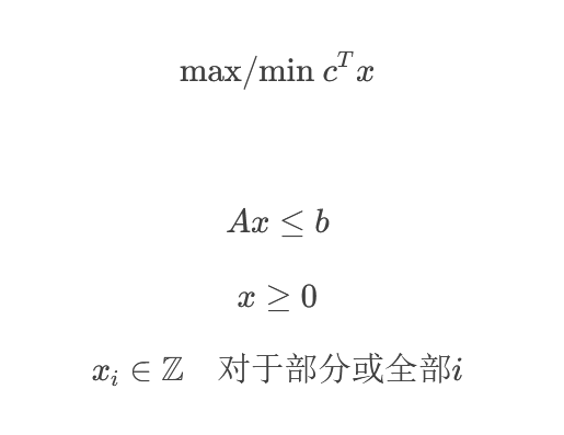
整數規劃（Integer Programming, IP）是數學規劃的一個分支，要求部分或全部決策變量取整數值。它是線性規劃的擴展，但增加了變量必須為整數的約束。

整數規劃的類型

純整數規劃：所有決策變量都必須取整數值
混合整數規劃：部分決策變量取整數值，其余可以是實數
0-1整數規劃：決策變量只能取0或1

最大化或最小化目標函數：

1. 分支定界法

最常用的整數規劃求解方法，通過系統地枚舉可行解的子集來尋找最優解。

2. 割平面法

通過添加額外的約束（割平面）來縮小可行域，逐步逼近整數解。

3. 啟發式算法

如遺傳算法、模擬退火等，用于求解大規模整數規劃問題。

以下是使用Python的PuLP庫求解整數規劃的完整示例：

import pulp
import numpy as np
import matplotlib.pyplot as plt
from matplotlib.patches import Polygondef solve_integer_programming():"""求解整數規劃問題的完整示例"""# 創建問題實例prob = pulp.LpProblem("Integer_Programming_Example", pulp.LpMaximize)# 定義決策變量 (必須為整數)x1 = pulp.LpVariable('x1', lowBound=0, cat='Integer')x2 = pulp.LpVariable('x2', lowBound=0, cat='Integer')# 定義目標函數prob += 3*x1 + 2*x2, "Objective Function"# 添加約束條件prob += 2*x1 + x2 <= 6, "Constraint 1"prob += x1 + 2*x2 <= 8, "Constraint 2"prob += x1 <= 2, "Constraint 3"prob += x2 <= 3, "Constraint 4"# 求解問題prob.solve()# 輸出結果print("Status:", pulp.LpStatus[prob.status])print("Optimal Solution:")for v in prob.variables():print(f"{v.name} = {v.varValue}")print(f"Optimal Value: {pulp.value(prob.objective)}")return probdef visualize_solution():"""可視化整數規劃問題的解"""# 定義約束條件x = np.linspace(0, 4, 100)# 約束1: 2x1 + x2 <= 6 → x2 <= 6 - 2x1y1 = 6 - 2*x# 約束2: x1 + 2x2 <= 8 → x2 <= (8 - x1)/2y2 = (8 - x)/2# 約束3: x1 <= 2# 約束4: x2 <= 3# 繪制約束條件plt.figure(figsize=(10, 8))plt.plot(x, y1, label=r'$2x_1 + x_2 \leq 6$')plt.plot(x, y2, label=r'$x_1 + 2x_2 \leq 8$')plt.axvline(x=2, color='green', linestyle='--', label=r'$x_1 \leq 2$')plt.axhline(y=3, color='purple', linestyle='--', label=r'$x_2 \leq 3$')# 繪制可行域vertices = np.array([[0, 0], [2, 0], [2, 2], [1, 3], [0, 3]])feasible_region = Polygon(vertices, alpha=0.3, color='gray')plt.gca().add_patch(feasible_region)# 標記整數點for i in range(0, 4):for j in range(0, 4):if (2*i + j <= 6) and (i + 2*j <= 8) and (i <= 2) and (j <= 3):plt.plot(i, j, 'ro', markersize=8)plt.text(i+0.05, j+0.05, f'({i},{j})', fontsize=10)# 標記最優解plt.plot(2, 2, 'go', markersize=10, label='Optimal Solution (2,2)')# 設置圖形屬性plt.xlim(0, 3.5)plt.ylim(0, 4)plt.xlabel(r'$x_1$')plt.ylabel(r'$x_2$')plt.title('Integer Programming Visualization')plt.legend()plt.grid(True, alpha=0.3)plt.show()def mixed_integer_example():"""混合整數規劃示例"""# 創建問題實例prob = pulp.LpProblem("Mixed_Integer_Example", pulp.LpMaximize)# 定義變量 (x1為整數，x2為連續變量)x1 = pulp.LpVariable('x1', lowBound=0, cat='Integer')x2 = pulp.LpVariable('x2', lowBound=0, cat='Continuous')# 目標函數prob += 4*x1 + 3*x2, "Objective"# 約束條件prob += 2*x1 + x2 <= 8, "Constraint1"prob += x1 + 2*x2 <= 7, "Constraint2"prob += x1 <= 3, "Constraint3"# 求解prob.solve()# 輸出結果print("\nMixed Integer Programming Results:")print("Status:", pulp.LpStatus[prob.status])for v in prob.variables():print(f"{v.name} = {v.varValue}")print(f"Optimal Value: {pulp.value(prob.objective)}")def binary_integer_example():"""0-1整數規劃示例 (背包問題)"""# 創建問題實例prob = pulp.LpProblem("Knapsack_Problem", pulp.LpMaximize)# 物品價值values = [10, 15, 40, 60, 20]# 物品重量weights = [1, 2, 4, 6, 3]# 背包容量capacity = 10# 創建0-1變量 (是否選擇物品)items = range(len(values))x = [pulp.LpVariable(f'x{i}', cat='Binary') for i in items]# 目標函數：最大化總價值prob += pulp.lpSum(values[i] * x[i] for i in items)# 約束條件：總重量不超過容量prob += pulp.lpSum(weights[i] * x[i] for i in items) <= capacity# 求解prob.solve()# 輸出結果print("\n0-1 Integer Programming (Knapsack Problem) Results:")print("Status:", pulp.LpStatus[prob.status])print("Selected items:")for i in items:if x[i].varValue == 1:print(f"Item {i+1} (Value: {values[i]}, Weight: {weights[i]})")print(f"Total Value: {pulp.value(prob.objective)}")print(f"Total Weight: {sum(weights[i] * x[i].varValue for i in items)}")if __name__ == "__main__":# 求解基本整數規劃問題problem = solve_integer_programming()# 可視化解visualize_solution()# 混合整數規劃示例mixed_integer_example()# 0-1整數規劃示例binary_integer_example()

1. 基本整數規劃求解

使用PuLP庫定義和求解整數規劃問題
包含目標函數和約束條件的定義
輸出最優解和目標函數值

2. 可視化

使用matplotlib繪制可行域和整數點
標記最優解位置
顯示所有約束條件

3. 混合整數規劃

演示同時包含整數和連續變量的情況
展示不同類型變量的定義方法

4. 0-1整數規劃

以背包問題為例展示0-1整數規劃
演示二進制變量的使用

安裝依賴

運行代碼前需要安裝以下Python庫：

pip install pulp numpy matplotlib

應用領域

整數規劃在現實世界中有廣泛應用：

物流與運輸：車輛路徑規劃、設施選址
生產計劃：排產優化、資源分配
金融：投資組合優化、風險管理
電信：網絡設計、頻率分配
能源：發電調度、電網優化

注意哦：

整數規劃通常是NP難問題，大規模問題可能需要專門的求解器；
對于復雜問題，可能需要使用商業求解器如Gurobi、CPLEX等；
啟發式算法可以用于求解大規模問題，但不能保證找到最優解。

3.動態規劃

動態規劃（Dynamic Programming，簡稱DP）是一種解決復雜問題的方法，它將問題分解為更小的子問題，并存儲子問題的解以避免重復計算。

動態規劃的核心思想

最優子結構：一個問題的最優解包含其子問題的最優解
重疊子問題：在遞歸求解過程中，相同的子問題會被多次計算
記憶化存儲：存儲已解決的子問題答案，避免重復計算

動態規劃的兩種實現方式

1. 自頂向下（記憶化搜索）

從原問題開始，遞歸地解決子問題
使用備忘錄存儲已計算的子問題結果

2. 自底向上（迭代法）

從最小的子問題開始，逐步構建到原問題的解
通常使用數組（DP表）來存儲子問題的解

經典問題：斐波那契數列

1. 遞歸解法（低效）

def fib_recursive(n):if n <= 1:return nreturn fib_recursive(n-1) + fib_recursive(n-2)

2. 記憶化搜索（自頂向下）

def fib_memo(n, memo=None):if memo is None:memo = {}if n in memo:return memo[n]if n <= 1:return nmemo[n] = fib_memo(n-1, memo) + fib_memo(n-2, memo)return memo[n]

3. 動態規劃（自底向上）

def fib_dp(n):if n <= 1:return n# 創建DP表dp = [0] * (n + 1)dp[0], dp[1] = 0, 1# 填充DP表for i in range(2, n + 1):dp[i] = dp[i-1] + dp[i-2]return dp[n]

4. 空間優化版本

def fib_optimized(n):if n <= 1:return nprev, curr = 0, 1for _ in range(2, n + 1):prev, curr = curr, prev + currreturn curr

經典問題：0-1背包問題

給定一組物品，每個物品有重量和價值，在不超過背包容量的情況下，選擇物品使得總價值最大。

def knapsack(weights, values, capacity):n = len(weights)# 創建DP表：dp[i][w] 表示前i個物品在容量為w時的最大價值dp = [[0] * (capacity + 1) for _ in range(n + 1)]# 填充DP表for i in range(1, n + 1):for w in range(capacity + 1):# 當前物品重量大于當前容量，不能選擇if weights[i-1] > w:dp[i][w] = dp[i-1][w]else:# 選擇當前物品或不選擇當前物品的最大值dp[i][w] = max(dp[i-1][w], dp[i-1][w - weights[i-1]] + values[i-1])return dp[n][capacity]# 示例
weights = [2, 3, 4, 5]
values = [3, 4, 5, 6]
capacity = 5
print(knapsack(weights, values, capacity))  # 輸出：7

動態規劃解題步驟

定義狀態：明確dp數組的含義
確定狀態轉移方程：找出如何從已知狀態推導出未知狀態
初始化：確定基礎情況的值
確定遍歷順序：確保在計算當前狀態時，所需的前置狀態已經計算完成
返回結果：返回最終需要的狀態值

完整示例：硬幣找零問題

給定不同面額的硬幣和一個總金額，計算湊成總金額所需的最少硬幣數。

def coin_change(coins, amount):# dp[i] 表示湊成金額i所需的最少硬幣數dp = [float('inf')] * (amount + 1)dp[0] = 0  # 金額為0時不需要任何硬幣for coin in coins:for i in range(coin, amount + 1):dp[i] = min(dp[i], dp[i - coin] + 1)return dp[amount] if dp[amount] != float('inf') else -1# 示例
coins = [1, 2, 5]
amount = 11
print(coin_change(coins, amount))  # 輸出：3 (5+5+1)

動態規劃的應用場景

最優化問題：求最大值、最小值
計數問題：求方案總數
存在性問題：判斷是否存在某種方案
序列問題：字符串、數組相關的子序列、子數組問題

動態規劃是一種強大的算法設計技術，通過將復雜問題分解為簡單的子問題，并避免重復計算來提高效率。掌握動態規劃需要：

理解最優子結構和重疊子問題的概念
熟練使用記憶化搜索和DP表兩種實現方式
通過大量練習來培養識別DP問題和設計狀態轉移方程的能力

4.圖論算法（Dijkstra、Floyd）

Dijkstra 算法（單源最短路徑）

Dijkstra 算法用于計算圖中單個源點到其他所有節點的最短路徑。它采用貪心策略，每次選擇當前已知最短路徑的節點進行擴展。

算法步驟

初始化：設置距離數組 dist[]，源點距離為 0，其他為無窮大
創建未訪問節點集合
當未訪問集合非空時：
- 選擇當前距離最小的未訪問節點 u
- 標記 u 為已訪問
- 更新 u 的所有未訪問鄰居的距離：如果通過 u 到達鄰居的路徑更短，則更新

時間復雜度

使用優先隊列：O((V+E)logV)
使用數組：O(V2)

代碼實現

import heapq
import sysdef dijkstra(graph, start):"""Dijkstra 算法實現參數:graph: 鄰接表表示的圖，graph[i] = [(j, weight), ...]start: 起始節點返回:dist: 從起始點到各點的最短距離prev: 前驅節點數組，用于重建路徑"""n = len(graph)dist = [sys.maxsize] * n  # 初始化距離為無窮大dist[start] = 0prev = [-1] * n  # 記錄前驅節點visited = [False] * n# 使用優先隊列 (距離, 節點)heap = [(0, start)]while heap:current_dist, u = heapq.heappop(heap)if visited[u]:continuevisited[u] = Truefor v, weight in graph[u]:if not visited[v]:new_dist = current_dist + weightif new_dist < dist[v]:dist[v] = new_distprev[v] = uheapq.heappush(heap, (new_dist, v))return dist, prevdef reconstruct_path(prev, start, end):"""根據前驅數組重建路徑"""path = []current = endwhile current != -1:path.append(current)current = prev[current]path.reverse()return path if path[0] == start else []# 示例使用
if __name__ == "__main__":# 創建示例圖 (有向圖)# 節點0到節點1的權重為4，節點0到節點2的權重為2，等等graph = [[(1, 4), (2, 2)],      # 節點0[(2, 5), (3, 10)],     # 節點1[(1, 1), (3, 8)],      # 節點2[(4, 2)],              # 節點3[(3, 5)]               # 節點4]start_node = 0dist, prev = dijkstra(graph, start_node)print("從節點", start_node, "出發的最短距離:")for i in range(len(dist)):path = reconstruct_path(prev, start_node, i)print(f"到節點{i}: 距離={dist[i]}, 路徑={path}")

Floyd-Warshall 算法（多源最短路徑）

Floyd 算法用于計算圖中所有節點對之間的最短路徑。它基于動態規劃，通過中間節點來逐步優化路徑。

定義 dp[k][i][j] = 從 i 到 j 且只經過節點 0..k 的最短路徑長度
狀態轉移方程：dp[k][i][j] = min(dp[k-1][i][j], dp[k-1][i][k] + dp[k-1][k][j])

初始化距離矩陣：對角線為0，有邊則為權重，無邊則為無窮大
對于每個中間節點 k：
- 對于每對節點 (i, j)：
  - 如果通過 k 的路徑更短，則更新距離

時間復雜度:O(V3)

def floyd_warshall(graph):"""Floyd-Warshall 算法實現參數:graph: 鄰接矩陣表示的圖，graph[i][j] = 權重，無邊時為無窮大返回:dist: 所有節點對之間的最短距離矩陣next_node: 用于重建路徑的下一節點矩陣"""n = len(graph)# 初始化距離矩陣和下一節點矩陣dist = [[0] * n for _ in range(n)]next_node = [[-1] * n for _ in range(n)]# 復制圖到距離矩陣，并初始化下一節點for i in range(n):for j in range(n):dist[i][j] = graph[i][j]if graph[i][j] != float('inf') and i != j:next_node[i][j] = j# 動態規劃過程for k in range(n):for i in range(n):if dist[i][k] == float('inf'):continuefor j in range(n):# 如果通過k的路徑更短，則更新if dist[i][k] + dist[k][j] < dist[i][j]:dist[i][j] = dist[i][k] + dist[k][j]next_node[i][j] = next_node[i][k]return dist, next_nodedef reconstruct_floyd_path(next_node, start, end):"""根據next_node矩陣重建路徑"""if next_node[start][end] == -1:return []path = [start]while start != end:start = next_node[start][end]path.append(start)return path# 示例使用
if __name__ == "__main__":# 創建示例圖的鄰接矩陣# 使用 float('inf') 表示無窮大n = 5  # 節點數量graph = [[float('inf')] * n for _ in range(n)]# 初始化對角線為0for i in range(n):graph[i][i] = 0# 添加邊graph[0][1] = 4graph[0][2] = 2graph[1][2] = 5graph[1][3] = 10graph[2][1] = 1graph[2][3] = 8graph[3][4] = 2graph[4][3] = 5dist, next_node = floyd_warshall(graph)print("所有節點對之間的最短距離:")for i in range(n):for j in range(n):if i != j:path = reconstruct_floyd_path(next_node, i, j)print(f"從{i}到{j}: 距離={dist[i][j]}, 路徑={path}")

算法比較

特性	Dijkstra	Floyd-Warshall
問題類型	單源最短路徑	多源最短路徑
圖類型	有向/無向，非負權重	有向/無向，可處理負權重（但無負環）
圖類型	有向/無向，非負權重	有向/無向，可處理負權重（但無負環）
空間復雜度	O(V+E)	O(V2)
適用場景	單源問題，稀疏圖	多源問題，稠密圖

Dijkstra 不能處理負權重邊，因為貪心策略會失效
Floyd 可以檢測負環：如果發現某個 dist[i][i] < 0，說明存在負環
對于稀疏圖，多次運行 Dijkstra 可能比 Floyd 更高效
實際應用中可根據具體需求選擇合適的算法

5.遺傳算法

遺傳算法（Genetic Algorithm, GA）是一種模擬自然選擇和遺傳學機制的優化算法。它通過模擬生物進化過程中的"適者生存"原則來搜索最優解。

遺傳算法的基本流程

初始化種群：隨機生成一組初始解（個體）
評估適應度：計算每個個體的適應度值
選擇：根據適應度選擇優秀的個體
交叉：將選中的個體進行交叉操作，產生新個體
變異：對新個體進行變異操作
重復：重復步驟2-5直到滿足終止條件

Python完整實現

下面是一個解決函數優化問題的遺傳算法完整實現：

import numpy as np
import matplotlib.pyplot as plt
from typing import List, Callable, Tupleclass GeneticAlgorithm:def __init__(self, objective_func: Callable, population_size: int = 100,chromosome_length: int = 10,crossover_rate: float = 0.8,mutation_rate: float = 0.01,elitism_count: int = 2,bounds: Tuple[float, float] = (-10, 10)):"""初始化遺傳算法參數:objective_func: 目標函數（適應度函數）population_size: 種群大小chromosome_length: 染色體長度（基因數量）crossover_rate: 交叉概率mutation_rate: 變異概率elitism_count: 精英保留數量bounds: 變量的取值范圍"""self.objective_func = objective_funcself.population_size = population_sizeself.chromosome_length = chromosome_lengthself.crossover_rate = crossover_rateself.mutation_rate = mutation_rateself.elitism_count = elitism_countself.bounds = bounds# 初始化種群self.population = self.initialize_population()self.best_individual = Noneself.best_fitness = float('-inf')self.fitness_history = []def initialize_population(self) -> np.ndarray:"""初始化種群 - 隨機生成二進制編碼的染色體"""return np.random.randint(0, 2, size=(self.population_size, self.chromosome_length))def decode_chromosome(self, chromosome: np.ndarray) -> float:"""將二進制染色體解碼為實際數值"""# 將二進制轉換為十進制decimal_value = int(''.join(map(str, chromosome)), 2)# 映射到指定范圍min_bound, max_bound = self.boundsvalue = min_bound + decimal_value * (max_bound - min_bound) / (2**self.chromosome_length - 1)return valuedef calculate_fitness(self, chromosome: np.ndarray) -> float:"""計算適應度值"""x = self.decode_chromosome(chromosome)return self.objective_func(x)def select_parents(self, fitness_values: np.ndarray) -> List[np.ndarray]:"""輪盤賭選擇父代"""# 確保適應度值為正min_fitness = np.min(fitness_values)if min_fitness < 0:fitness_values = fitness_values - min_fitness + 1e-6# 計算選擇概率total_fitness = np.sum(fitness_values)probabilities = fitness_values / total_fitness# 選擇父代selected_indices = np.random.choice(len(self.population), size=self.population_size - self.elitism_count, p=probabilities,replace=True)return [self.population[i] for i in selected_indices]def crossover(self, parent1: np.ndarray, parent2: np.ndarray) -> Tuple[np.ndarray, np.ndarray]:"""單點交叉"""if np.random.rand() < self.crossover_rate:# 隨機選擇交叉點crossover_point = np.random.randint(1, self.chromosome_length - 1)# 執行交叉child1 = np.concatenate([parent1[:crossover_point], parent2[crossover_point:]])child2 = np.concatenate([parent2[:crossover_point], parent1[crossover_point:]])return child1, child2else:return parent1.copy(), parent2.copy()def mutate(self, chromosome: np.ndarray) -> np.ndarray:"""位翻轉變異"""mutated_chromosome = chromosome.copy()for i in range(len(mutated_chromosome)):if np.random.rand() < self.mutation_rate:mutated_chromosome[i] = 1 - mutated_chromosome[i]  # 翻轉位return mutated_chromosomedef evolve(self, generations: int = 100):"""執行進化過程"""for generation in range(generations):# 計算適應度fitness_values = np.array([self.calculate_fitness(ind) for ind in self.population])# 記錄最佳個體best_idx = np.argmax(fitness_values)current_best_fitness = fitness_values[best_idx]if current_best_fitness > self.best_fitness:self.best_fitness = current_best_fitnessself.best_individual = self.population[best_idx].copy()self.fitness_history.append(self.best_fitness)# 選擇精英elite_indices = np.argsort(fitness_values)[-self.elitism_count:]elites = [self.population[i] for i in elite_indices]# 選擇父代parents = self.select_parents(fitness_values)# 交叉和變異產生新種群new_population = []# 添加精英new_population.extend(elites)# 生成后代for i in range(0, len(parents), 2):if i + 1 < len(parents):parent1, parent2 = parents[i], parents[i+1]child1, child2 = self.crossover(parent1, parent2)new_population.append(self.mutate(child1))new_population.append(self.mutate(child2))# 確保種群大小不變self.population = np.array(new_population[:self.population_size])# 打印進度if generation % 10 == 0:best_x = self.decode_chromosome(self.best_individual)print(f"Generation {generation}: Best Fitness = {self.best_fitness:.6f}, Best x = {best_x:.6f}")def get_best_solution(self) -> Tuple[float, float]:"""獲取最佳解"""best_x = self.decode_chromosome(self.best_individual)return best_x, self.best_fitnessdef plot_progress(self):"""繪制進化過程"""plt.figure(figsize=(10, 6))plt.plot(self.fitness_history)plt.title('Evolution of Best Fitness')plt.xlabel('Generation')plt.ylabel('Fitness')plt.grid(True)plt.show()# 示例：尋找函數 f(x) = -x^2 + 10 的最大值
def objective_function(x):return -x**2 + 10# 運行遺傳算法
if __name__ == "__main__":# 初始化遺傳算法ga = GeneticAlgorithm(objective_func=objective_function,population_size=50,chromosome_length=20,crossover_rate=0.9,mutation_rate=0.01,elitism_count=2,bounds=(-10, 10))# 運行進化ga.evolve(generations=100)# 獲取結果best_x, best_fitness = ga.get_best_solution()print(f"\n最佳解: x = {best_x:.6f}, f(x) = {best_fitness:.6f}")# 繪制進化過程ga.plot_progress()# 驗證結果print(f"理論最大值在 x=0 處，f(0)=10")print(f"實際找到的最大值在 x={best_x:.6f} 處，f(x)={best_fitness:.6f}")

更復雜的示例：多變量優化

# 多變量優化示例：尋找函數 f(x, y) = -x^2 - y^2 + 10 的最大值class MultiVariableGA:def __init__(self, objective_func: Callable,num_variables: int = 2,population_size: int = 100,chromosome_length_per_var: int = 10,crossover_rate: float = 0.8,mutation_rate: float = 0.01,elitism_count: int = 2,bounds: List[Tuple[float, float]] = [(-10, 10), (-10, 10)]):self.objective_func = objective_funcself.num_variables = num_variablesself.chromosome_length_per_var = chromosome_length_per_varself.total_chromosome_length = num_variables * chromosome_length_per_varself.bounds = boundsself.ga = GeneticAlgorithm(objective_func=self._evaluate,population_size=population_size,chromosome_length=self.total_chromosome_length,crossover_rate=crossover_rate,mutation_rate=mutation_rate,elitism_count=elitism_count,bounds=(0, 1)  # 占位值，實際解碼在_evaluate中處理)def _evaluate(self, chromosome: np.ndarray) -> float:"""解碼染色體并評估適應度"""variables = []for i in range(self.num_variables):start_idx = i * self.chromosome_length_per_varend_idx = start_idx + self.chromosome_length_per_varvar_chromosome = chromosome[start_idx:end_idx]# 解碼單個變量decimal_value = int(''.join(map(str, var_chromosome)), 2)min_bound, max_bound = self.bounds[i]value = min_bound + decimal_value * (max_bound - min_bound) / (2**self.chromosome_length_per_var - 1)variables.append(value)return self.objective_func(*variables)def evolve(self, generations: int = 100):"""執行進化"""self.ga.evolve(generations)def get_best_solution(self):"""獲取最佳解"""best_chromosome = self.ga.best_individualvariables = []for i in range(self.num_variables):start_idx = i * self.chromosome_length_per_varend_idx = start_idx + self.chromosome_length_per_varvar_chromosome = best_chromosome[start_idx:end_idx]decimal_value = int(''.join(map(str, var_chromosome)), 2)min_bound, max_bound = self.bounds[i]value = min_bound + decimal_value * (max_bound - min_bound) / (2**self.chromosome_length_per_var - 1)variables.append(value)best_fitness = self.ga.best_fitnessreturn variables, best_fitness# 定義多變量目標函數
def multi_var_objective(x, y):return -x**2 - y**2 + 10# 運行多變量遺傳算法
if __name__ == "__main__":multi_ga = MultiVariableGA(objective_func=multi_var_objective,num_variables=2,population_size=100,chromosome_length_per_var=15,crossover_rate=0.85,mutation_rate=0.02,bounds=[(-5, 5), (-5, 5)])multi_ga.evolve(generations=100)best_vars, best_fitness = multi_ga.get_best_solution()print(f"\n最佳解: x = {best_vars[0]:.6f}, y = {best_vars[1]:.6f}, f(x,y) = {best_fitness:.6f}")print(f"理論最大值在 (0,0) 處，f(0,0)=10")

遺傳算法的關鍵參數調優

種群大小：太小的種群可能無法充分探索搜索空間，太大的種群會增加計算成本
交叉率：控制交叉操作的概率，通常設置在0.6-0.9之間
變異率：通常設置較低的值（0.001-0.1），以避免破壞好的解
選擇策略：除了輪盤賭選擇，還可以使用錦標賽選擇、排名選擇等
編碼方式：除了二進制編碼，還可以使用實數編碼、排列編碼等

應用領域

遺傳算法廣泛應用于：

函數優化
機器學習參數調優
調度問題
路徑規劃
神經網絡設計
圖像處理

6.蟻群算法

蟻群算法(Ant Colony Optimization, ACO)是一種模擬螞蟻覓食行為的群體智能優化算法。螞蟻在尋找食物源時會釋放信息素，其他螞蟻能夠感知這種信息素并傾向于跟隨信息素濃度較高的路徑，從而形成一種正反饋機制。

信息素：螞蟻在路徑上釋放的化學物質，濃度越高表示路徑越優
啟發式信息：反映路徑的直觀吸引力（如距離的倒數）
狀態轉移規則：螞蟻選擇下一個節點的概率公式
信息素更新：包括揮發和增強兩個過程

算法步驟

初始化參數和信息素矩陣
將螞蟻放置在起始點
每只螞蟻根據狀態轉移規則構建完整路徑
計算每條路徑的成本（如總距離）
更新信息素矩陣
重復步驟2-5直到滿足終止條件

Python完整實現

下面以解決旅行商問題(TSP)為例實現蟻群算法：

import numpy as np
import matplotlib.pyplot as plt
import randomclass AntColonyOptimization:def __init__(self, distances, n_ants, n_best, n_iterations, decay, alpha=1, beta=1):"""初始化蟻群算法參數參數:distances: 城市間距離矩陣n_ants: 螞蟻數量n_best: 每輪保留的最佳路徑數量n_iterations: 迭代次數decay: 信息素揮發率alpha: 信息素重要程度參數beta: 啟發式信息重要程度參數"""self.distances = distancesself.pheromone = np.ones(self.distances.shape) / len(distances)self.all_inds = range(len(distances))self.n_ants = n_antsself.n_best = n_bestself.n_iterations = n_iterationsself.decay = decayself.alpha = alphaself.beta = betadef run(self):"""運行蟻群算法"""best_path = Nonebest_distance = float('inf')best_paths = []best_distances = []for iteration in range(self.n_iterations):all_paths = self.gen_all_paths()self.spread_pheromone(all_paths, self.n_best)# 更新最佳路徑shortest_path = min(all_paths, key=lambda x: x[1])if shortest_path[1] < best_distance:best_path = shortest_path[0]best_distance = shortest_path[1]best_paths.append(best_path)best_distances.append(best_distance)# 信息素揮發self.pheromone *= (1 - self.decay)if iteration % 10 == 0:print(f"迭代次數 {iteration}: 最佳距離 = {best_distance}")return best_path, best_distance, best_paths, best_distancesdef gen_path_dist(self, path):"""計算路徑總距離"""total_dist = 0for i in range(len(path)):total_dist += self.distances[path[i-1]][path[i]]return total_distdef gen_all_paths(self):"""所有螞蟻生成路徑"""all_paths = []for _ in range(self.n_ants):path = self.gen_path(0)  # 從城市0開始all_paths.append((path, self.gen_path_dist(path)))return all_pathsdef gen_path(self, start):"""單只螞蟻生成路徑"""path = [start]visited = set([start])while len(visited) < len(self.distances):probs = self.gen_move_probs(path[-1], visited)next_city = self.choose_next_city(probs)path.append(next_city)visited.add(next_city)return pathdef gen_move_probs(self, current, visited):"""生成移動到下一個城市的概率"""pheromone = np.copy(self.pheromone[current])pheromone[list(visited)] = 0  # 已訪問城市概率設為0# 計算啟發式信息（距離的倒數）heuristic = np.zeros(len(self.distances))for i in range(len(heuristic)):if i not in visited and self.distances[current][i] != 0:heuristic[i] = 1 / self.distances[current][i]# 計算概率分子numerator = (pheromone ** self.alpha) * (heuristic ** self.beta)# 歸一化概率if np.sum(numerator) == 0:# 如果所有概率都為0，隨機選擇未訪問城市unvisited = [i for i in self.all_inds if i not in visited]prob = np.zeros(len(self.distances))for city in unvisited:prob[city] = 1return prob / np.sum(prob)return numerator / np.sum(numerator)def choose_next_city(self, probs):"""根據概率選擇下一個城市"""return np.random.choice(self.all_inds, 1, p=probs)[0]def spread_pheromone(self, all_paths, n_best):"""更新信息素"""# 按路徑長度排序sorted_paths = sorted(all_paths, key=lambda x: x[1])# 只對最佳路徑釋放信息素for path, dist in sorted_paths[:n_best]:for i in range(len(path)):current_city = path[i]next_city = path[(i + 1) % len(path)]# 信息素增量與路徑長度成反比self.pheromone[current_city][next_city] += 1 / distself.pheromone[next_city][current_city] += 1 / dist# 生成示例數據：隨機城市坐標
def generate_cities(n_cities):np.random.seed(42)cities = np.random.rand(n_cities, 2) * 100return cities# 計算城市間距離矩陣
def calculate_distances(cities):n = len(cities)distances = np.zeros((n, n))for i in range(n):for j in range(n):if i != j:distances[i][j] = np.sqrt((cities[i][0] - cities[j][0])**2 + (cities[i][1] - cities[j][1])**2)return distances# 可視化結果
def plot_results(cities, best_path, best_distances):fig, (ax1, ax2) = plt.subplots(1, 2, figsize=(15, 5))# 繪制最佳路徑ax1.plot(cities[best_path, 0], cities[best_path, 1], 'o-')ax1.set_xlabel('X坐標')ax1.set_ylabel('Y坐標')ax1.set_title(f'最佳路徑 (總距離: {best_distances[-1]:.2f})')# 繪制收斂曲線ax2.plot(best_distances)ax2.set_xlabel('迭代次數')ax2.set_ylabel('最短距離')ax2.set_title('收斂曲線')ax2.grid(True)plt.tight_layout()plt.show()# 主函數
def main():# 參數設置n_cities = 20n_ants = 30n_best = 5n_iterations = 100decay = 0.1alpha = 1beta = 2# 生成數據cities = generate_cities(n_cities)distances = calculate_distances(cities)# 運行蟻群算法aco = AntColonyOptimization(distances, n_ants, n_best, n_iterations, decay, alpha, beta)best_path, best_distance, best_paths, best_distances = aco.run()print(f"\n最終最佳路徑: {best_path}")print(f"最終最短距離: {best_distance}")# 可視化結果plot_results(cities, best_path, best_distances)if __name__ == "__main__":main()

螞蟻數量：一般為城市數量的1-2倍
信息素揮發率(decay)：0.1-0.5之間，避免過早收斂
α和β參數：
- α控制信息素影響（通常1-2）
- β控制啟發式信息影響（通常2-5）
迭代次數：根據問題復雜度調整，通常100-1000次

算法優缺點

優點：

強大的全局搜索能力
正反饋機制促進優良解的發現
易于并行化處理
適用于離散優化問題

缺點：

收斂速度較慢
參數調節復雜
容易陷入局部最優（需配合局部搜索）

應用領域

旅行商問題(TSP)
車輛路徑問題(VRP)
作業車間調度
網絡路由優化
數據挖掘中的聚類分析

二、預測模型

1.ARIMA模型

ARIMA（Autoregressive Integrated Moving Average），全稱為自回歸積分滑動平均模型。它是時間序列預測中最經典、最常用的方法之一，尤其適用于處理非平穩序列。

1. 核心思想

ARIMA模型的核心思想是：將非平穩時間序列轉化為平穩時間序列，然后將因變量僅對其滯后值以及隨機誤差項的現值和滯后值進行回歸所建立的模型。

2. 模型結構：ARIMA(p, d, q)

模型由三個部分組成，對應三個參數 (p, d, q)：

AR(p) - 自回歸部分 (Autoregressive)
- 含義：描述當前值與歷史值之間的關系。用變量自身的歷史時間數據來預測自己。
- 模型：$X_t = c + \sum_{i=1}^{p} \phi_i X_{t-i} + \epsilon_t$
- 參數 p：自回歸項的階數，表示用過去多少期的數據來預測當前值。可以通過偏自相關函數(PACF) 圖來確定。
I(d) - 差分部分 (Integrated)
- 含義：將非平穩時間序列轉換為平穩序列的過程。差分可以消除數據中的趨勢和季節性。
- 操作：d階差分就是計算d次相鄰觀測值之間的差值。
  - 1階差分：$X’t = X_t - X{t-1}$
  - 2階差分：$X’’t = X’t - X’{t-1} = (X_t - X{t-1}) - (X_{t-1} - X_{t-2})$
- 參數 d：使序列變為平穩所需的最小差分階數。通常通過ADF檢驗（單位根檢驗） 來確定。
MA(q) - 移動平均部分 (Moving Average)
- 含義：描述當前值與歷史預測誤差之間的關系。它捕捉的是時間序列中隨機沖擊的效應。
- 模型：$X_t = \mu + \epsilon_t + \sum_{i=1}^{q} \theta_i \epsilon_{t-i}$
- 參數 q：移動平均項的階數，表示模型使用過去多少個預測誤差。可以通過自相關函數(ACF) 圖來確定。

綜合模型ARIMA(p, d, q)：
對原始序列進行d階差分后，得到的新序列遵循ARMA(p, q)模型。
$\Delta^d X_t = c + \sum_{i=1}^{p} \phi_i \Delta^d X_{t-i} + \epsilon_t + \sum_{i=1}^{q} \theta_i \epsilon_{t-i}$
其中，$\Delta^d$ 是d階差分算子。

3. 建模步驟

序列平穩化 (確定d)
- 繪制原始序列圖，觀察是否有明顯趨勢或季節性。
- 進行ADF單位根檢驗。如果p-value > 0.05，則認為序列不平穩，需要進行差分。
- 重復差分和ADF檢驗，直到序列平穩，記錄差分次數 d。
確定p和q
- 對平穩化后的序列繪制ACF（自相關圖） 和PACF（偏自相關圖）。
- ACF圖：拖尾（逐漸衰減到0）還是截尾（快速降為0）。
- PACF圖：拖尾還是截尾。
- 粗略判斷準則：
  - p的確定：看PACF圖。如果PACF在滯后p階后截尾（突然趨于0），則p可以取該值。
  - q的確定：看ACF圖。如果ACF在滯后q階后截尾，則q可以取該值。
- 更精確的方法是使用網格搜索（Grid Search），根據AIC（Akaike Information Criterion） 或BIC（Bayesian Information Criterion） 準則來選擇模型，AIC/BIC越小越好。
參數估計
- 使用最大似然估計（MLE）等方法來確定AR和MA項的系數 ($\phi_i$, $\theta_i$)。
模型診斷
- 殘差分析：一個好的ARIMA模型的殘差應該是一個白噪聲（均值為0，方差恒定，無自相關）。
  - 繪制殘差圖，觀察是否在0附近隨機波動。
  - 對殘差進行Ljung-Box檢驗，如果p-value很大（>0.05），則不能拒絕殘差是白噪聲的原假設，說明模型擬合良好。
預測
- 使用擬合好的模型進行未來值的預測。

4.Python

我們將使用經典的AirPassengers（航空公司乘客）數據集來演示。

1. 導入必要庫

import numpy as np
import pandas as pd
import matplotlib.pyplot as plt
%matplotlib inline# 統計模型
from statsmodels.tsa.stattools import adfuller # ADF檢驗
from statsmodels.graphics.tsaplots import plot_acf, plot_pacf # ACF/PACF圖
from statsmodels.tsa.arima.model import ARIMA # ARIMA模型# 評估指標
from sklearn.metrics import mean_squared_error, mean_absolute_error
import warnings
warnings.filterwarnings('ignore') # 忽略警告信息

2. 加載數據并探索

# 加載數據
url = "https://raw.githubusercontent.com/jbrownlee/Datasets/master/airline-passengers.csv"
data = pd.read_csv(url, parse_dates=['Month'], index_col='Month')
data.index.freq = 'MS' # 設置頻率為“月起始”（Month Start）
series = data['Passengers']# 查看數據
print(series.head())
plt.figure(figsize=(12, 5))
plt.plot(series)
plt.title('AirPassengers Dataset')
plt.xlabel('Year')
plt.ylabel('Passengers')
plt.grid(True)
plt.show()

3. 序列平穩化 - 確定參數d

# 定義ADF檢驗函數
def adf_test(series):result = adfuller(series)print('ADF Statistic: %f' % result[0])print('p-value: %f' % result[1])print('Critical Values:')for key, value in result[4].items():print('\t%s: %.3f' % (key, value))if result[1] <= 0.05:print("-> p-value <= 0.05. Reject the null hypothesis. Data is stationary.")else:print("-> p-value > 0.05. Fail to reject the null hypothesis. Data is non-stationary.")# 對原始序列進行ADF檢驗
print("ADF Test for Original Series:")
adf_test(series)# 進行1階差分并再次檢驗
series_diff_1 = series.diff().dropna()
print("\nADF Test after 1st Order Differencing:")
adf_test(series_diff_1)# 繪制差分后的序列
plt.figure(figsize=(12, 5))
plt.plot(series_diff_1)
plt.title('AirPassengers After 1st Order Differencing')
plt.grid(True)
plt.show()

輸出：原始序列p值很大，非平穩。1階差分后p值可能仍然>0.05（因為還有季節性），但對于演示，我們通常取d=1。對于有強季節性的數據，需要使用SARIMA（季節性ARIMA），但這里我們先按簡單ARIMA處理，取d=1。

4. 確定參數p和q

# 對平穩化后的序列（差分后）繪制ACF和PACF圖
fig, (ax1, ax2) = plt.subplots(2, 1, figsize=(12, 8))# ACF圖
plot_acf(series_diff_1, lags=40, ax=ax1)
ax1.set_title('Autocorrelation Function (ACF)')# PACF圖
plot_pacf(series_diff_1, lags=40, ax=ax2, method='ywm') # 使用 ywm 方法避免警告
ax2.set_title('Partial Autocorrelation Function (PACF)')plt.tight_layout()
plt.show()

更嚴謹的方法是使用網格搜索確定p和q：

# 網格搜索尋找最佳p, q組合 (d已固定為1)
# 定義p, d, q參數的取值范圍
p_range = range(0, 4)  # 0 to 3
q_range = range(0, 4)  # 0 to 3
d = 1best_aic = np.inf
best_order = Nonefor p in p_range:for q in q_range:try:model = ARIMA(series, order=(p, d, q))results = model.fit()aic = results.aicif aic < best_aic:best_aic = aicbest_order = (p, d, q)print(f'ARIMA({p},{d},{q}) - AIC: {aic:.2f}')except Exception as e:print(f'Error fitting ARIMA({p},{d},{q}): {e}')continueprint(f'\nBest Model Order: ARIMA{best_order} with AIC: {best_aic:.2f}')

5. 擬合ARIMA模型

# 使用確定的參數 (p,d,q) 擬合模型
# 這里我們使用 (2, 1, 1)，請根據你的網格搜索結果修改
p, d, q = 2, 1, 1model = ARIMA(series, order=(p, d, q))
model_fit = model.fit()# 輸出模型摘要
print(model_fit.summary())

6. 模型診斷 - 殘差分析

# 繪制殘差圖
residuals = model_fit.resid
plt.figure(figsize=(12, 5))
plt.plot(residuals)
plt.title('Residuals from ARIMA Model')
plt.grid(True)
plt.show()# 殘差的ACF圖
plot_acf(residuals, lags=40)
plt.title('ACF of Residuals')
plt.show()# Ljung-Box檢驗 (查看殘差是否為白噪聲)
from statsmodels.stats.diagnostic import acorr_ljungbox
lb_test = acorr_ljungbox(residuals, lags=10, return_df=True)
print("Ljung-Box test results for residuals:")
print(lb_test)# 如果所有p-value都很大(>0.05)，說明殘差是白噪聲，模型OK

7. 預測

# 劃分訓練集和測試集 (最后24個月作為測試集)
split_point = len(series) - 24
train, test = series.iloc[:split_point], series.iloc[split_point:]# 在訓練集上重新擬合模型
model_train = ARIMA(train, order=(p, d, q))
model_train_fit = model_train.fit()# 進行預測
# start: 預測開始的索引
# end: 預測結束的索引
# dynamic: False 表示使用一步預測（更準確但可能滯后）
forecast = model_train_fit.get_prediction(start=len(train), end=len(series)-1, dynamic=False)
forecast_values = forecast.predicted_mean
forecast_ci = forecast.conf_int() # 置信區間# 計算評估指標
mse = mean_squared_error(test, forecast_values)
rmse = np.sqrt(mse)
mae = mean_absolute_error(test, forecast_values)
print(f'\nTest MSE: {mse:.2f}')
print(f'Test RMSE: {rmse:.2f}')
print(f'Test MAE: {mae:.2f}')# 繪制結果
plt.figure(figsize=(14, 7))
plt.plot(train, label='Training Data')
plt.plot(test, label='Actual Test Data', color='blue')
plt.plot(forecast_values, color='red', label='Forecast')
# 繪制置信區間
plt.fill_between(forecast_ci.index,forecast_ci.iloc[:, 0],forecast_ci.iloc[:, 1], color='pink', alpha=0.3, label='95% Confidence Interval')
plt.title('ARIMA Model Forecast vs Actuals')
plt.legend()
plt.grid(True)
plt.show()

8. 預測未來（未知）數據

# 使用全部數據重新擬合最終模型
final_model = ARIMA(series, order=(p, d, q))
final_model_fit = final_model.fit()# 預測未來12個月
forecast_steps = 12
forecast_future = final_model_fit.get_forecast(steps=forecast_steps)
forecast_future_values = forecast_future.predicted_mean
forecast_future_ci = forecast_future.conf_int()# 創建未來時間的索引
future_index = pd.date_range(series.index[-1] + pd.DateOffset(months=1), periods=forecast_steps, freq='MS')# 繪制歷史數據和未來預測
plt.figure(figsize=(14, 7))
plt.plot(series, label='Historical Data')
plt.plot(future_index, forecast_future_values, color='green', label='Future Forecast')
plt.fill_between(future_index,forecast_future_ci.iloc[:, 0],forecast_future_ci.iloc[:, 1], color='lightgreen', alpha=0.3, label='95% Confidence Interval')
plt.title(f'ARIMA{best_order} Forecast for Next {forecast_steps} Months')
plt.legend()
plt.grid(True)
plt.show()# 打印預測值
print("\nFuture Forecast Values:")
print(pd.DataFrame({'Date': future_index, 'Forecasted_Passengers': forecast_future_values.values}).round(1))

2.SARIMA模型

SARIMA（Seasonal AutoRegressive Integrated Moving Average）模型是ARIMA模型的擴展，專門用于處理帶有季節性（Seasonality）成分的時間序列數據。它結合了非季節性的ARIMA模型和季節性成分的模型。

一個完整的SARIMA模型通常表示為： SARIMA(p, d, q)×(P, D, Q, s)

讓我們來分解這個復雜的符號：

1. 非季節性部分 (p, d, q)

這與標準ARIMA模型完全相同：

p (自回歸項 - AR): 表示模型中使用的自身滯后觀測值的數量。它捕捉當前值與過去值之間的關系（例如：昨天的銷售額可能影響今天的銷售額）。
d (差分次數 - I): 為了使時間序列平穩化（即均值、方差不隨時間變化）所需的差分次數。一階差分即用當前值減去前一個值 (Y_t - Y_{t-1})。
q (移動平均項 - MA): 表示模型中使用的過去滯后預測誤差的數量。它捕捉歷史預測誤差對當前值的影響。

2. 季節性部分 (P, D, Q, s)

這是SARIMA獨有的部分，用于建模季節性模式：

P (季節性自回歸項): 類似于p，但它使用的是季節性周期滯后的觀測值。例如，對于月度數據，P=1可能會使用去年同月的值來預測今年這個月的值。
D (季節性差分次數): 為了使序列的季節性成分平穩化所需的季節性差分次數。季節性差分即用當前值減去上一個周期的對應值。例如，月度數據的季節性一階差分為 Y_t - Y_{t-12}。
Q (季節性移動平均項): 類似于q，但它使用的是季節性周期滯后的預測誤差。
s (季節周期長度): 這是最關鍵的參數，定義了季節循環的長度。
- 月度數據： s = 12
- 季度數據： s = 4
- 日度數據（周周期）： s = 7
- 小時數據（天周期）： s = 24

模型的思想

SARIMA模型的核心思想是：一個時間序列可以分解為趨勢性（由p,d,q部分建模）和季節性（由P,D,Q,s部分建模）兩部分。通過差分（d和D）消除不平穩的趨勢和季節因素后，再用自回歸（p和P）和移動平均（q和Q）模型來捕捉剩下的序列相關性。

Python完整代碼實現

我們將使用經典的航空乘客數據集（Air Passengers）來演示，這是一個具有明顯趨勢和12個月季節性的月度數據。

步驟 1：導入必要的庫

import numpy as np
import pandas as pd
import matplotlib.pyplot as plt
from statsmodels.tsa.statespace.sarimax import SARIMAX
from statsmodels.tsa.seasonal import seasonal_decompose
from statsmodels.tsa.stattools import adfuller
from statsmodels.graphics.tsaplots import plot_acf, plot_pacf
from sklearn.metrics import mean_squared_error, mean_absolute_error
import warnings
warnings.filterwarnings('ignore') # 忽略警告信息，使輸出更清晰# 設置繪圖風格
plt.style.use('ggplot')

步驟 2：加載和探索數據

# 加載數據
url = "https://raw.githubusercontent.com/jbrownlee/Datasets/master/airline-passengers.csv"
data = pd.read_csv(url, parse_dates=['Month'], index_col='Month')
data.index.freq = 'MS' # 非常重要！設置索引頻率為“月初”（Month Start）# 重命名列
data.columns = ['Passengers']# 查看數據
print(data.head())
print("\n數據信息:")
print(data.info())# 繪制時間序列圖
plt.figure(figsize=(12, 5))
plt.plot(data)
plt.title('Monthly Airline Passengers (1949-1960)')
plt.xlabel('Date')
plt.ylabel('Number of Passengers')
plt.show()

步驟 3：時間序列分解

# 進行加法分解 (如果季節波動幅度不隨時間變化，也可以用乘法‘multiplicative’)
result = seasonal_decompose(data['Passengers'], model='multiplicative') # 此數據更適合乘法模型# 繪制分解結果
fig = result.plot()
fig.set_size_inches(12, 8)
plt.show()

步驟 4：平穩性檢驗 - ADF test

# 定義ADF檢驗函數
def adf_test(series):result = adfuller(series)print('ADF Statistic: %f' % result[0])print('p-value: %f' % result[1])print('Critical Values:')for key, value in result[4].items():print('\t%s: %.3f' % (key, value))if result[1] <= 0.05:print("-> 拒絕原假設，序列是平穩的。")else:print("-> 無法拒絕原假設，序列是非平穩的。")print("原始序列的ADF檢驗:")
adf_test(data['Passengers'])

步驟 5：差分處理

為了使序列平穩，我們需要進行差分。通常先進行一階常規差分消除趨勢，再進行一階季節性差分（周期s=12）消除季節性。

# 一階常規差分
data['1st_Diff'] = data['Passengers'].diff(1)
# 季節性差分 (周期為12)
data['Seasonal_Diff'] = data['Passengers'].diff(12)# 繪制差分后的序列
fig, axes = plt.subplots(2, 1, figsize=(12, 8))
axes[0].plot(data['1st_Diff'])
axes[0].set_title('First Order Differencing')
axes[1].plot(data['Seasonal_Diff'])
axes[1].set_title('Seasonal Differencing (s=12)')
plt.tight_layout()
plt.show()# 對“一階常規差分+一階季節性差分”后的數據進行ADF檢驗
# 先drop掉NaN值
combined_diff = data['Passengers'].diff(1).diff(12).dropna()
print("\n‘一階常規+一階季節性’差分后的ADF檢驗:")
adf_test(combined_diff)

步驟 6：確定模型參數 (p, q, P, Q)

通過觀察自相關圖(ACF)和偏自相關圖(PACF)來確定 p, q, P, Q 的大致范圍。

# 對平穩化后的序列（即雙重差分后的數據）繪制ACF和PACF圖
fig, axes = plt.subplots(2, 1, figsize=(12, 8))# ACF圖
plot_acf(combined_diff, lags=40, ax=axes[0])
axes[0].set_title('ACF for Stationary Series')# PACF圖
plot_pacf(combined_diff, lags=40, ax=axes[1], method='ywm') # ‘ywm’是Method的推薦值
axes[1].set_title('PACF for Stationary Series')plt.tight_layout()
plt.show()

非季節性參數 (p, q):
- 看最初幾個滯后點（lag 1, 2, 3...）。
- PACF在lag 1和2后截尾（顯著超出藍色區域），提示 p 可能為 1 或 2。
- ACF在lag 1后拖尾（逐漸衰減），提示 q 可能為 0 或 1。
季節性參數 (P, Q):
- 看季節性滯后點（lag 12, 24, 36...）。
- PACF在lag 12處有一個顯著的尖峰，提示 P 可能為 1。
- ACF在lag 12處有一個顯著的尖峰，提示 Q 可能為 1。

步驟 7：擬合SARIMA模型

# 定義模型參數
p, d, q = 1, 1, 1
P, D, Q, s = 1, 1, 1, 12# 劃分訓練集和測試集 (例如，最后24個月作為測試集)
train_size = int(len(data) * 0.8)
train, test = data['Passengers'][:train_size], data['Passengers'][train_size:]
print(f"訓練集大小: {len(train)}")
print(f"測試集大小: {len(test)}")# 創建并擬合SARIMAX模型 (Statsmodels中使用SARIMAX)
model = SARIMAX(train,order=(p, d, q),         # 非季節性部分 (p, d, q)seasonal_order=(P, D, Q, s), # 季節性部分 (P, D, Q, s)enforce_stationarity=False,enforce_invertibility=False)# 擬合模型
model_fit = model.fit(disp=False) # disp=False減少輸出# 輸出模型總結
print(model_fit.summary())

步驟 8：模型診斷

# 繪制模型診斷圖
model_fit.plot_diagnostics(figsize=(12, 8))
plt.show()

解讀診斷圖：

標準化殘差圖：應該沒有明顯的趨勢或季節性。
殘差直方圖：應該近似服從正態分布（鐘形曲線）。
*正態Q-Q圖：點應大致分布在45度線上。*
殘差ACF圖：沒有任何自相關（所有滯后點都在置信區間內）。如果ACF圖良好，說明模型已經充分捕捉了數據中的信息。

步驟 9：進行預測并評估

# 進行樣本內動態預測和樣本外預測
# ‘dynamic=False’意味著樣本內預測使用全部歷史信息
pred_dynamic = model_fit.get_prediction(start=pd.to_datetime('1958-01-01'), dynamic=False, full_results=True)
pred_dynamic_ci = pred_dynamic.conf_int() # 獲取預測的置信區間# 獲取樣本外預測（對未來時間的預測），這里預測測試集之后12個月
forecast_steps = len(test)
forecast_obj = model_fit.get_forecast(steps=forecast_steps)
forecast = forecast_obj.predicted_mean
forecast_ci = forecast_obj.conf_int()# 將預測結果轉換為Series，方便繪圖
forecast_series = pd.Series(forecast, index=test.index)
lower_series = pd.Series(forecast_ci.iloc[:, 0], index=test.index)
upper_series = pd.Series(forecast_ci.iloc[:, 1], index=test.index)# 繪制所有數據、預測值和置信區間
plt.figure(figsize=(12, 6))# 繪制歷史數據
plt.plot(data['Passengers'], label='Observed')# 繪制樣本外預測值
plt.plot(forecast_series, color='r', label='Forecast')# 繪制置信區間
plt.fill_between(forecast_series.index, lower_series, upper_series, color='pink', alpha=0.3)plt.title('SARIMA Forecast: Air Passengers')
plt.xlabel('Date')
plt.ylabel('Number of Passengers')
plt.legend(loc='upper left')
plt.show()# 計算評估指標 (RMSE and MAE)
rmse = np.sqrt(mean_squared_error(test, forecast))
mae = mean_absolute_error(test, forecast)
print(f"測試集 RMSE: {rmse:.2f}")
print(f"測試集 MAE: {mae:.2f}")

步驟 10（可選）：自動化尋找最佳參數

手動解讀ACF/PACF很繁瑣。我們可以使用pmdarima庫的auto_arima函數自動搜索最佳參數。

# 首先需要安裝 pmdarima
# pip install pmdarima

from pmdarima import auto_arima# 使用auto_arima自動尋找最佳參數 (這會運行一段時間)
stepwise_model = auto_arima(data['Passengers'],start_p=0, start_q=0,max_p=3, max_q=3,start_P=0, start_Q=0,max_P=3, max_Q=3,m=12, # 季節周期sseasonal=True,d=None, D=None, # 讓模型自動判斷d, Dtrace=True, # 打印搜索過程error_action='ignore',suppress_warnings=True,stepwise=True) # 使用逐步搜索算法，更快print(stepwise_model.summary())
# 最佳模型參數會打印出來，然后你可以用這個參數重新擬合模型

總結

理解數據：可視化并檢查趨勢和季節性。
平穩化：通過差分（常規和季節性）使序列平穩，確定 d 和 D。
確定參數：通過ACF/PACF圖初步判斷 p, q, P, Q，或使用auto_arima自動搜索。
擬合模型：使用SARIMAX函數擬合模型。
模型診斷：檢查殘差是否為隨機白噪聲。
預測評估：進行預測并用量化指標（如RMSE）評估模型性能。

3.線性回歸模型

線性回歸是一種通過擬合自變量（X）和因變量（y）之間的線性關系來進行預測的監督學習算法。它的目標是找到一條直線（或一個超平面），使得所有數據點到這條直線的距離的平方和最小。

1. 模型表示

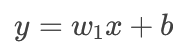
對于最簡單的一元線性回歸（一個特征），模型方程表示為：

其中：

$y$ 是預測值（目標變量）。
$x$ 是特征（自變量）。
$w_1$ 是權重（Weight），也就是斜率。
$b$ 是偏置（Bias），也就是截距。

對于更一般的多元線性回歸（多個特征），模型方程表示為：

我們可以用向量形式更簡潔地表示。令 $\mathbf{w} = [w_1, w_2, ..., w_n]^T$, $\mathbf{x} = [x_1, x_2, ..., x_n]^T$，則：

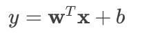
為了簡化計算，通常我們會將 $b$ 也并入權重向量 $\mathbf{w}$ 中。我們添加一個恒為 1 的特征 $x_0$，令 $w_0 = b$，那么公式就變成了：

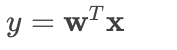
其中 $\mathbf{w} = [w_0, w_1, w_2, ..., w_n]^T$, $\mathbf{x} = [1, x_1, x_2, ..., x_n]^T$。

3. 損失函數 (Loss Function)

如何找到最優的 $\mathbf{w}$？我們需要一個標準來衡量模型預測的好壞，這個標準就是損失函數。

線性回歸最常用的損失函數是均方誤差 (MSE)。它是所有樣本的預測值 $\hat{y}^{(i)}$ 與真實值 $y^{(i)}$ 之差的平方和的平均值。

其中 $m$ 是樣本數量。

我們的目標就是找到一組參數 $\mathbf{w^*}$，使得損失函數 $J(\mathbf{w})$ 最小化。

4. 求解方法：最小二乘法 (Ordinary Least Squares)

最小化 MSE 損失函數有兩種主要方法：

a) 正規方程 (Normal Equation) - 閉式解
通過直接對損失函數求導并令導數為零，可以推導出一個解析解（直接計算公式）：

其中：

$\mathbf{X}$ 是一個 $m \times (n+1)$ 的矩陣（包含了 $x_0=1$ 這一列）。
$\mathbf{y}$ 是一個 $m \times 1$ 的向量，包含所有真實標簽。

優點：不需要選擇學習率，一次計算即可得到最優解。
缺點：當特征數量 $n$ 非常大時（例如 >10000），計算矩陣的逆 $(X^TX)^{-1}$ 會非常慢，甚至不可行。

b) 梯度下降 (Gradient Descent) - 迭代解

這是一種迭代優化算法，適用于特征數量很大的情況。

核心思想：從一組隨機的 $\mathbf{w}$ 開始，反復迭代，每次沿著損失函數下降最快的方向（即梯度負方向）更新 $\mathbf{w}$，逐步逼近最小值。

權重更新公式：

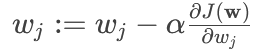
其中 $\alpha$ 是學習率，控制每一步的步長。

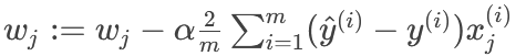
對 MSE 損失函數求偏導，得到具體的更新公式：

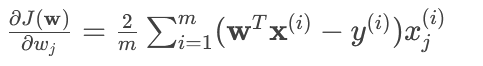
所以對于每個 $w_j$：

優點：在特征數量很大時也能很好地工作。
缺點：需要選擇學習率 $\alpha$，可能需要多次迭代才能收斂。

Python 完整實現

我們將實現兩種方法：1. 正規方程 和 2. 梯度下降。

1. 導入必要的庫

import numpy as np
import matplotlib.pyplot as plt
from sklearn.model_selection import train_test_split
from sklearn.datasets import make_regression
from sklearn.metrics import mean_squared_error, r2_score
from sklearn.preprocessing import StandardScaler

2. 生成模擬數據

# 生成線性回歸數據集
np.random.seed(42) # 確保結果可重現
X, y = make_regression(n_samples=100, n_features=1, noise=20, random_state=42)# 劃分訓練集和測試集
X_train, X_test, y_train, y_test = train_test_split(X, y, test_size=0.2, random_state=42)# 可視化數據
plt.figure(figsize=(8, 6))
plt.scatter(X, y, alpha=0.7, c='blue', edgecolors='k', label='Data Points')
plt.title('Generated Regression Data')
plt.xlabel('Feature (X)')
plt.ylabel('Target (y)')
plt.legend()
plt.grid(True, linestyle='--', alpha=0.7)
plt.show()

3. 方法一：使用正規方程實現

class LinearRegressionNormalEquation:def __init__(self):self.w = None # 權重參數self.b = None # 偏置參數（為了清晰，單獨表示）def fit(self, X, y):# 為X添加一列1，用于計算偏置項b (即w0)X_b = np.c_[np.ones((X.shape[0], 1)), X] # [1, X]# 計算正規方程的解: w = (X^T * X)^(-1) * X^T * y# 使用np.linalg.pinv求偽逆，比inv更穩定，尤其在X^T.X接近奇異矩陣時self.w = np.linalg.pinv(X_b.T.dot(X_b)).dot(X_b.T).dot(y)# 將權重向量分解為偏置b和權重wself.b = self.w[0]self.w = self.w[1:]def predict(self, X):# 模型預測: y_pred = X * w + breturn X.dot(self.w) + self.b# 使用模型
model_ne = LinearRegressionNormalEquation()
model_ne.fit(X_train, y_train)
y_pred_ne = model_ne.predict(X_test)# 評估模型
mse_ne = mean_squared_error(y_test, y_pred_ne)
r2_ne = r2_score(y_test, y_pred_ne)
print(f"正規方程模型 - MSE: {mse_ne:.2f}, R2: {r2_ne:.4f}")# 可視化擬合結果
plt.figure(figsize=(8, 6))
plt.scatter(X, y, alpha=0.7, c='blue', edgecolors='k', label='Data Points')
x_line = np.linspace(X.min(), X.max(), 100).reshape(-1, 1)
y_line = model_ne.predict(x_line)
plt.plot(x_line, y_line, color='red', linewidth=3, label='Fitted Line (Normal Eq.)')
plt.title('Linear Regression using Normal Equation')
plt.xlabel('Feature (X)')
plt.ylabel('Target (y)')
plt.legend()
plt.grid(True, linestyle='--', alpha=0.7)
plt.show()

4. 方法二：使用梯度下降實現

class LinearRegressionGradientDescent:def __init__(self, learning_rate=0.01, n_iters=1000):self.learning_rate = learning_rateself.n_iters = n_itersself.w = Noneself.b = 0self.loss_history = [] # 記錄每次迭代的損失值def fit(self, X, y):m, n = X.shape# 初始化參數self.w = np.zeros(n)self.b = 0# 梯度下降迭代for i in range(self.n_iters):# 計算當前預測值y_pred = np.dot(X, self.w) + self.b# 計算誤差 (y_pred - y)error = y_pred - y# 計算梯度dw = (2/m) * np.dot(X.T, error)db = (2/m) * np.sum(error)# 更新參數self.w -= self.learning_rate * dwself.b -= self.learning_rate * db# 記錄當前迭代的損失 (MSE)loss = np.mean(error ** 2)self.loss_history.append(loss)# 可選：每100次迭代打印一次損失# if i % 100 == 0:#     print(f"Iteration {i}, Loss: {loss:.4f}")def predict(self, X):return np.dot(X, self.w) + self.b# 注意：梯度下降對特征縮放敏感，最好先進行標準化
scaler = StandardScaler()
X_train_scaled = scaler.fit_transform(X_train)
X_test_scaled = scaler.transform(X_test)# 使用模型
model_gd = LinearRegressionGradientDescent(learning_rate=0.1, n_iters=1000)
model_gd.fit(X_train_scaled, y_train)
y_pred_gd = model_gd.predict(X_test_scaled)# 評估模型
mse_gd = mean_squared_error(y_test, y_pred_gd)
r2_gd = r2_score(y_test, y_pred_gd)
print(f"梯度下降模型 - MSE: {mse_gd:.2f}, R2: {r2_gd:.4f}")# 可視化損失下降曲線
plt.figure(figsize=(8, 5))
plt.plot(range(model_gd.n_iters), model_gd.loss_history)
plt.title('Gradient Descent - Loss over Iterations')
plt.xlabel('Iterations')
plt.ylabel('Mean Squared Error Loss')
plt.grid(True, linestyle='--', alpha=0.7)
plt.show()# 可視化擬合結果 (需要將標準化的X轉換回原始尺度進行繪圖)
plt.figure(figsize=(8, 6))
plt.scatter(X, y, alpha=0.7, c='blue', edgecolors='k', label='Data Points')
x_line = np.linspace(X.min(), X.max(), 100).reshape(-1, 1)
x_line_scaled = scaler.transform(x_line) # 將繪圖用的X也標準化
y_line = model_gd.predict(x_line_scaled)
plt.plot(x_line, y_line, color='green', linewidth=3, label='Fitted Line (Gradient Descent)')
plt.title('Linear Regression using Gradient Descent')
plt.xlabel('Feature (X)')
plt.ylabel('Target (y)')
plt.legend()
plt.grid(True, linestyle='--', alpha=0.7)
plt.show()

5. 與 Scikit-Learn 的實現進行對比

from sklearn.linear_model import LinearRegression# 使用Scikit-Learn的線性回歸（默認使用正規方程）
model_sklearn = LinearRegression()
model_sklearn.fit(X_train, y_train)
y_pred_sk = model_sklearn.predict(X_test)# 評估模型
mse_sk = mean_squared_error(y_test, y_pred_sk)
r2_sk = r2_score(y_test, y_pred_sk)
print(f"Scikit-Learn模型 - MSE: {mse_sk:.2f}, R2: {r2_sk:.4f}")# 比較我們實現的模型和Scikit-Learn的系數
print("\n系數比較:")
print(f"正規方程實現: w = {model_ne.w[0]:.4f}, b = {model_ne.b:.4f}")
print(f"Scikit-Learn實現: w = {model_sklearn.coef_[0]:.4f}, b = {model_sklearn.intercept_:.4f}")

總結與關鍵點

核心概念：線性回歸通過最小化預測值與真實值之間的均方誤差（MSE） 來找到最佳擬合直線。
兩種解法：
- 正規方程：直接、精確，適合特征數較少（<10000）的數據集。
- 梯度下降：迭代、通用，適合特征數非常多或數據集巨大的情況，但需要調整學習率和迭代次數。
特征縮放：在使用梯度下降法時，對特征進行標準化（Standardization）或歸一化（Normalization）至關重要，這可以大大加快收斂速度。正規方程則不需要。
評估指標：常用 MSE（均方誤差） 和 R2 Score（決定系數） 來評估模型性能。R2 越接近 1，說明模型擬合得越好。
我們的實現 vs Scikit-Learn：你應該會看到我們自己實現的模型與 Scikit-Learn 的結果幾乎完全相同，這驗證了我們代碼的正確性。