背景

雖然模型基本都是表格數據那一套了，算法都沒什么新鮮點，但是本次數據還是很值得寫個案例的，有征信數據，各種，個人，機構，逾期匯總.....

這么多特征來做機器學習模型應該還不錯。本次帶來，在實際生產業務中，拿到一大堆的表，怎么對這些數據進行合并，清洗整理，特征工程，然后機器學習建模，評估模型效果。

---

數據介紹

本次數據主要分這么多表格：

"contest_basic
（基礎表-數據集）"
"contest_ext_crd_hd_report
(機構版征信-報告主表)"

"contest_ext_crd_cd_ln
（機構版征信-貸款）"

"contest_ext_crd_cd_lnd
（機構版征信-貸記卡）"

"contest_ext_crd_is_creditcue
（機構版征信-信用提示）"

"contest_ext_crd_is_sharedebt
（機構版征信-未銷戶貸記卡或者未結清貸款）"

"contest_ext_crd_is_ovdsummary
（機構版征信-逾期(透支)信息匯總）"

"contest_ext_crd_qr_recordsmr
（機構版征信-查詢記錄匯總）"

"contest_ext_crd_qr_recorddtlinfo
（機構版征信-信貸審批查詢記錄明細）"

"contest_ext_crd_cd_ln_spl?
（機構版征信-貸款特殊交易）"

"contest_ext_crd_cd_lnd_ovd
（機構版征信-貸記卡逾期/透支記錄）"

表格里面都有各種的詳細的字段

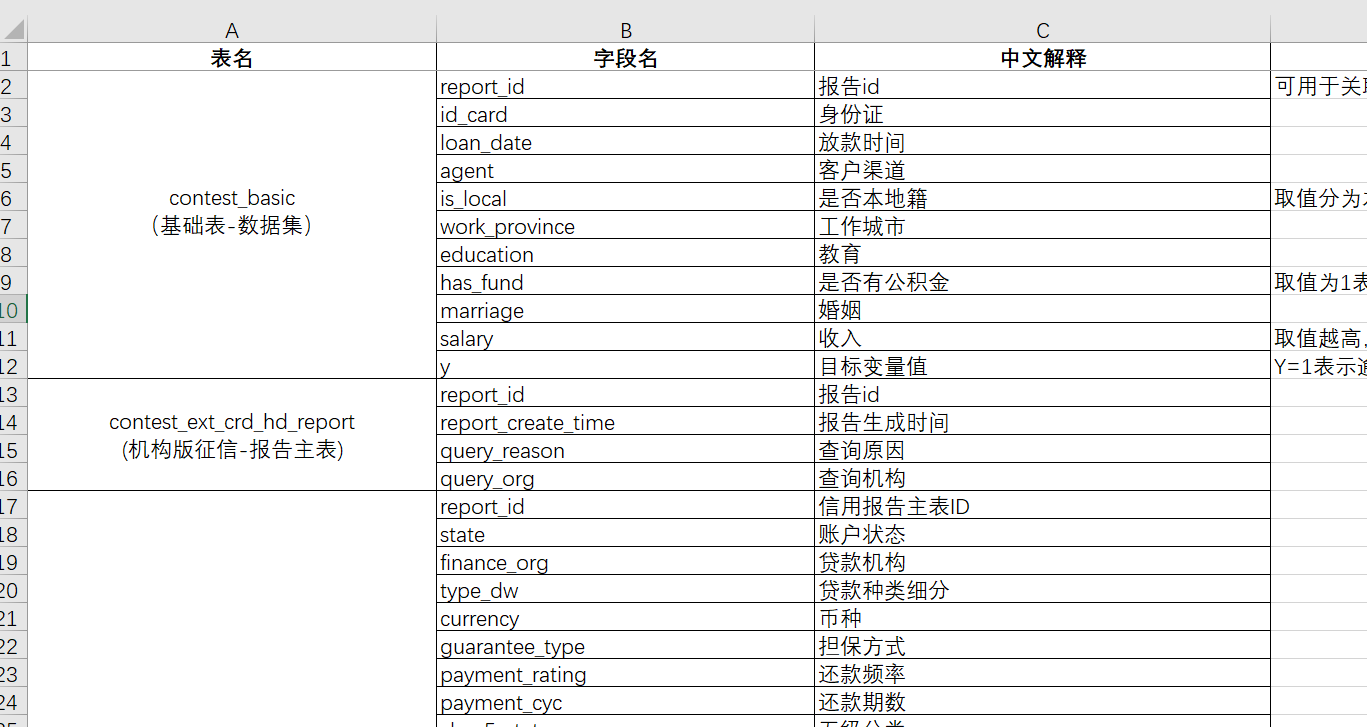
太多了就不詳細列舉了。數據都放在了“原始數據”這個文件夾里面方便下面代碼讀取。

當然需要本文的全部案例數據和代碼文件的同學還是可以參考：征信風控

實驗過程與結果

• 數據預處理（空值處理、異常值處理、變量標注、獨熱編碼......）
• 數據可視化
• 特征工程
• 實驗過程
• 實驗結果

---

代碼實現

下面開始寫代碼吧

導入包

import numpy as np
import pandas as pd
import matplotlib.pyplot as plt
import seaborn as sns
import os,randomplt.rcParams["font.sans-serif"] = ["SimHei"]  # 設置顯示中文字體
plt.rcParams["axes.unicode_minus"] = False  # 設置正常顯示符號

數據的合并整理?

讀取合并數據文件，由于這個數據里面的征信不同，來源的數據集太多，所以文件會很亂，做機器學習首先得把他們這些數據都合并一起，就得做很多清洗和處理，下面就開始這樣合并和整理的過程。

#查看數據文件夾里面的所有數據文件的名稱
data_lis=os.listdir('原始數據')
data_lis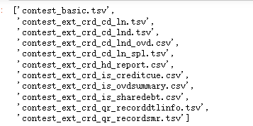

#循環讀取所有數據，放入列表?

def read_and_merge_files(folder_path):# 用于存儲所有數據框的列表dataframes = []# 遍歷文件夾中的所有文件for filename in os.listdir(folder_path):file_path = os.path.join(folder_path, filename)# 根據文件后綴使用不同的方法讀取if filename.endswith('.csv'):df = pd.read_csv(file_path)elif filename.endswith('.tsv'):df = pd.read_csv(file_path, sep='\t')else:continue  # 忽略非CSV/TSV文件df.columns=[c.lower() for c in df.columns]print(f"{filename}讀取完成，數據形狀為{df.shape}")dataframes.append(df)return dataframes

讀取所有的文件?

folder_path = '原始數據'  # 替換為文件夾路徑
dataframes_list = read_and_merge_files(folder_path)
len(dataframes_list)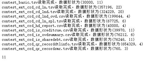

所有的數據合并需要按照report_id進行關聯，但是有的表可能report_id可能會重復，所以先查看一下

#查看數據信息，report_id有重復
def check_files(dataframes):# 確保至少有一個數據框if not dataframes:raise ValueError("No CSV or TSV files found in the directory.")# 依次檢查所有表的report_id數量for i,df in enumerate(dataframes):duplicates = df['report_id'].duplicated().sum()print(f'表{data_lis[i]}中重復的 report_id 數量: {duplicates}')

### 查看每個表的重復情況
?

check_files(dataframes_list)?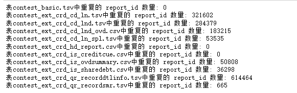

對這些重復數據選取最后一條進行合并，表示最新最近的情況

### 合并的時候不需要的字段就過濾掉

unuseless=["query_date","querier",'get_time',    #查詢，信息更新的日期"scheduled_payment_date", "scheduled_payment_amount", "actual_payment_amount", "recent_pay_date",  #本月、最近的應還什么的，沒有時效性，去掉"finance_org", "currency",  "open_date",'end_date',    #日期類都去掉'first_loan_open_month','first_loancard_open_month','first_sl_open_month', 'loan_date','month_dw','report_create_time','payment_state', #一些ID類，編碼類 也都去掉'id_card','loan_id','loancard_id','content' ]def merge_files(dataframes):# 使用第一個表（假設是contest_basic）作為左連接底表main_df = dataframes[0]for i,df in enumerate(dataframes[1:]):#按照report_id 去重保留最后一個df=df[[col for col in df.columns if col not in unuseless]]df=df.drop_duplicates(subset='report_id', keep='last')print(f'正在合并數據表：{data_lis[1:][i]}...')# 按照'report_id'列進行左連接name=data_lis[1:][i].split('_')[-1]main_df = pd.merge(main_df, df, on='report_id', how='left',suffixes=('', f'_@{name}')) ## 名稱重復的特征后面加上@和數據文件名稱print(f'合并之后的數據形狀{main_df.shape}')return main_df

使用這個函數

threshold = len(df_all) * 0.5df_all = df_all.dropna(axis=1, thresh=threshold)
df_all.shape

df_all=merge_files(dataframes_list)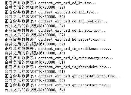

?# 刪除缺失率高達50%的列

threshold = len(df_all) * 0.5df_all = df_all.dropna(axis=1, thresh=threshold)
df_all.shape

### 去除一些 id列(唯一編碼，對模型沒有用)，設置report_id為索引
for c in ['id_card','loan_date','loan_id','loancard_id']:if c in df_all.columns:df_all.drop(c,axis=1,inplace=True)
df_all=df_all.set_index('report_id')

## 查看數據信息

df_all.info()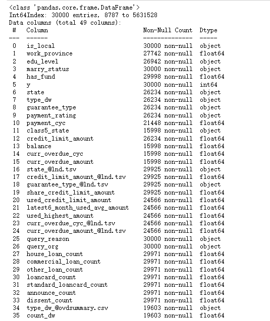

文本的變量很多，需要處理，我們首先查看文本變量的信息

### 查看文本變量的信息
df_all.select_dtypes(include='object').describe().T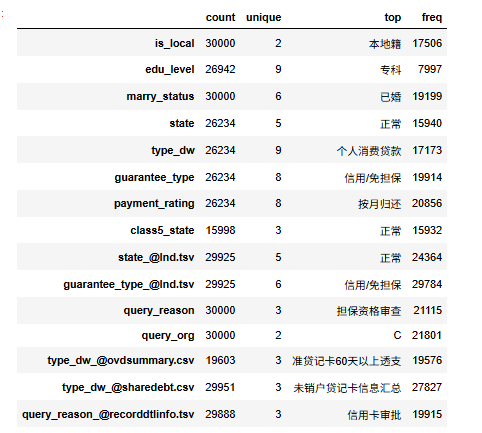

##查看字符變量名稱

str_columns=df_all.select_dtypes(include='object').columns.to_list()
str_columns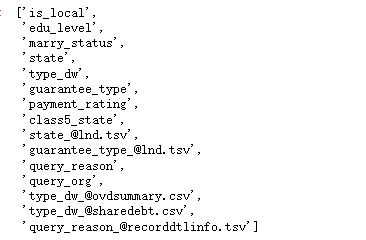

df_all.select_dtypes(exclude='object').describe().T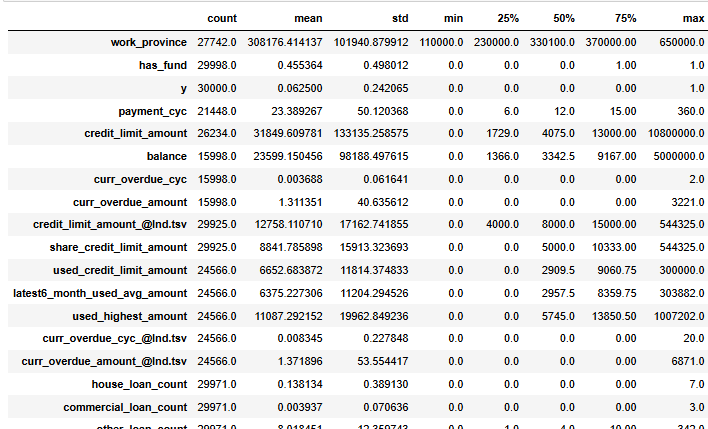

數據洗完了，儲存一下吧

### 查看了上述信息，數據合并沒問題，進行儲存
df_all.to_csv('合并后的數據.csv')

---

數據預處理

數據預處理（空值處理、異常值處理、變量標注、獨熱編碼......）

缺失值查看

### 讀取合并的數據

df=pd.read_csv('合并后的數據.csv').set_index('report_id')
df.head(3)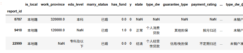

### 查看標簽y的比例?

df['y'].value_counts()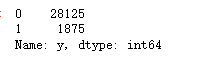

查看數據信息

df.info()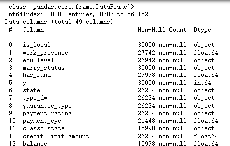

這樣看可能不全面不直觀，我們觀察缺失值情況直接畫圖就行了

#觀察缺失值
import missingno as msno
msno.matrix(df)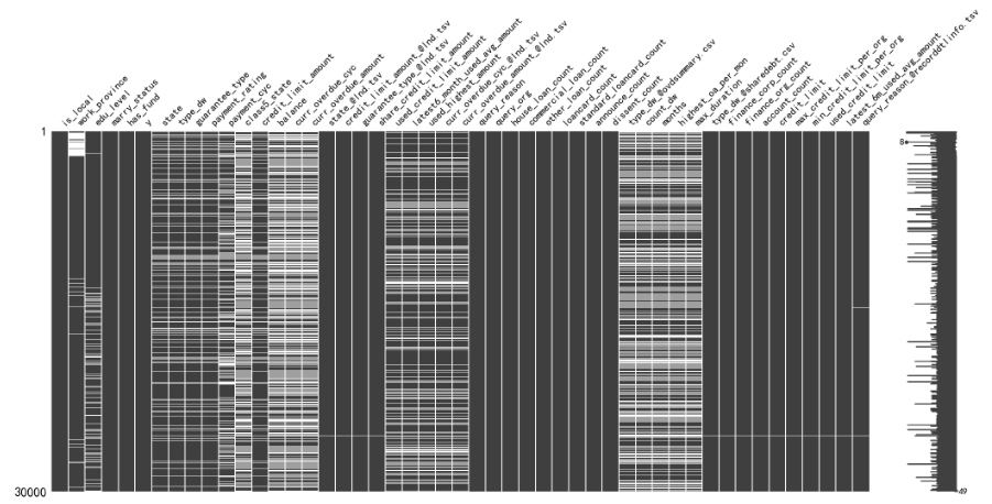

可以很清晰的看到哪些列的缺失率比較多，并且這些缺失都是某些樣本造成的，可能是合并數據的時候，某些人某些身份證沒有這一類的數據。

變量預處理

#取值唯一的變量刪除

for col in df.columns:if len(df[col].value_counts())==1:print(col)df.drop(col,axis=1,inplace=True)

這兩個變量取值唯一就刪除掉了。

#查看數值型數據,

#pd.set_option('display.max_columns', 30)
df.select_dtypes(exclude=['object']).describe()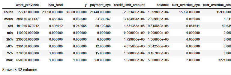

做機器學習當然需要特征越分散越好，因為這樣就可以在X上更加有區分度，從而更好的分類。所以那些數據分布很集中的變量可以扔掉。我們用異眾比例來衡量數據的分散程度

#計算異眾比例?

variation_ratio_s=0.05
for col in df.select_dtypes(exclude=['object']).columns:df_count=df[col].value_counts()kind=df_count.index[0]variation_ratio=1-(df_count.iloc[0]/len(df[col]))if variation_ratio<variation_ratio_s:print(f'{col} 最多的取值為{kind}，異眾比例為{round(variation_ratio,4)},太小了，沒區分度刪掉')df.drop(col,axis=1,inplace=True)

?

##查看非數值型數據
?

df.select_dtypes(exclude=['int64','float64']).describe()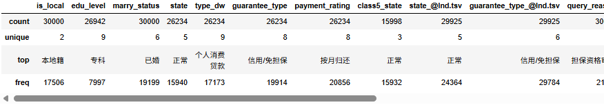

基本都是可以轉為類別型變量

空值處理

缺失值有很多填充方式，可以用中位數，均值，眾數。 也可以就采用那一行前面一個或者后面一個有效值去填充空的

#數值型變量使用均值填充
#文本型數據使用眾數填充
def fill_missing_values(df):# 選擇數值型變量并使用均值填充缺失值for col in df.select_dtypes(include=['int64', 'float64']).columns:mean_value = df[col].mean()df[col].fillna(mean_value, inplace=True)# 選擇字符型變量并使用眾數填充缺失值for col in df.select_dtypes(exclude=['int64', 'float64']).columns:mode_value = df[col].mode()[0]df[col].fillna(mode_value, inplace=True)return df
df=fill_missing_values(df)

查看數據信息

df.info()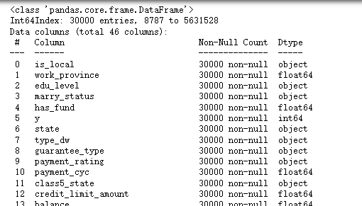

可以看到所有的變量沒有缺失值了。

異常值處理

主要是對數值型變量，查看是否有驗證的異常值處理

df_number=df.select_dtypes(include=['int64', 'float64'])

#X異常值處理，先標準化
from sklearn.preprocessing import StandardScaler
scaler = StandardScaler()
df_number_s = scaler.fit_transform(df_number)

可視化一下看看異常值

plt.figure(figsize=(20,8))
plt.boxplot(x=df_number_s,labels=df_number.columns)
#plt.hlines([-10,10],0,len(columns))
plt.show()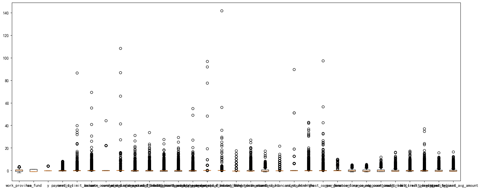

可以看到，很多變量都存在極大值，我們需要進行異常值處理

這個函數傳入三個參數，要處理的數據框，異常值多的變量列名，還有篩掉幾倍的方差。我下面選用的是10，也是就說如果一個樣本數據大于整體10倍的標準差之外就篩掉。

#異常值多的列進行處理
def deal_outline(data,col,n):   #數據，要處理的列名，幾倍的方差for c in col:mean=data[c].mean()std=data[c].std()data=data[(data[c]>mean-n*std)&(data[c]<mean+n*std)]#print(data.shape)return data

df_number=deal_outline(df_number,df_number.columns,10)
df_number.shape

?

### 處理完成后將數據篩選給原始數據
df=df.loc[df_number.index,:]
df.shape

?這樣，原始3w數據減少了594條

變量標注、獨熱編碼......

由于這里分類變量有點多，并且每個變量的類別的取值也較多，使用獨熱編碼可能造成維度災難，所以我們這里進行labelencode，因子化處理類別變量

df_category=df.copy()
#選出列表變量
categorical_feature=df.select_dtypes(include=['category','object']).columns.to_list()
for col in categorical_feature:df[col]=df[col].astype('category').cat.codes    #因子化
df.shape

df.info()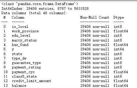  

可以看到所有的變量都變成數值型變量了，下面進行可視化

---

數據可視化

類別變量可視化

### 我們對類別變量畫柱狀圖
len(df_category.select_dtypes(exclude=['int64', 'float64']).columns)

# Select non-numeric columns
non_numeric_columns = df_category.select_dtypes(exclude=['int64', 'float64']).columns
f, axes = plt.subplots(4, 4, figsize=(14,14),dpi=256)
# Flatten axes for easy iterating
axes_flat = axes.flatten()
for i, column in enumerate(non_numeric_columns):if i < 15:  sns.countplot(x=column, data=df_category, ax=axes_flat[i])axes_flat[i].set_title(f'Count of {column}')for label in axes_flat[i].get_xticklabels():label.set_rotation(90)   #類別標簽旋轉一下，免得多了堆疊看不清# Hide any unused subplots
for j in range(i + 1, 15):f.delaxes(axes_flat[j])plt.tight_layout()
plt.show()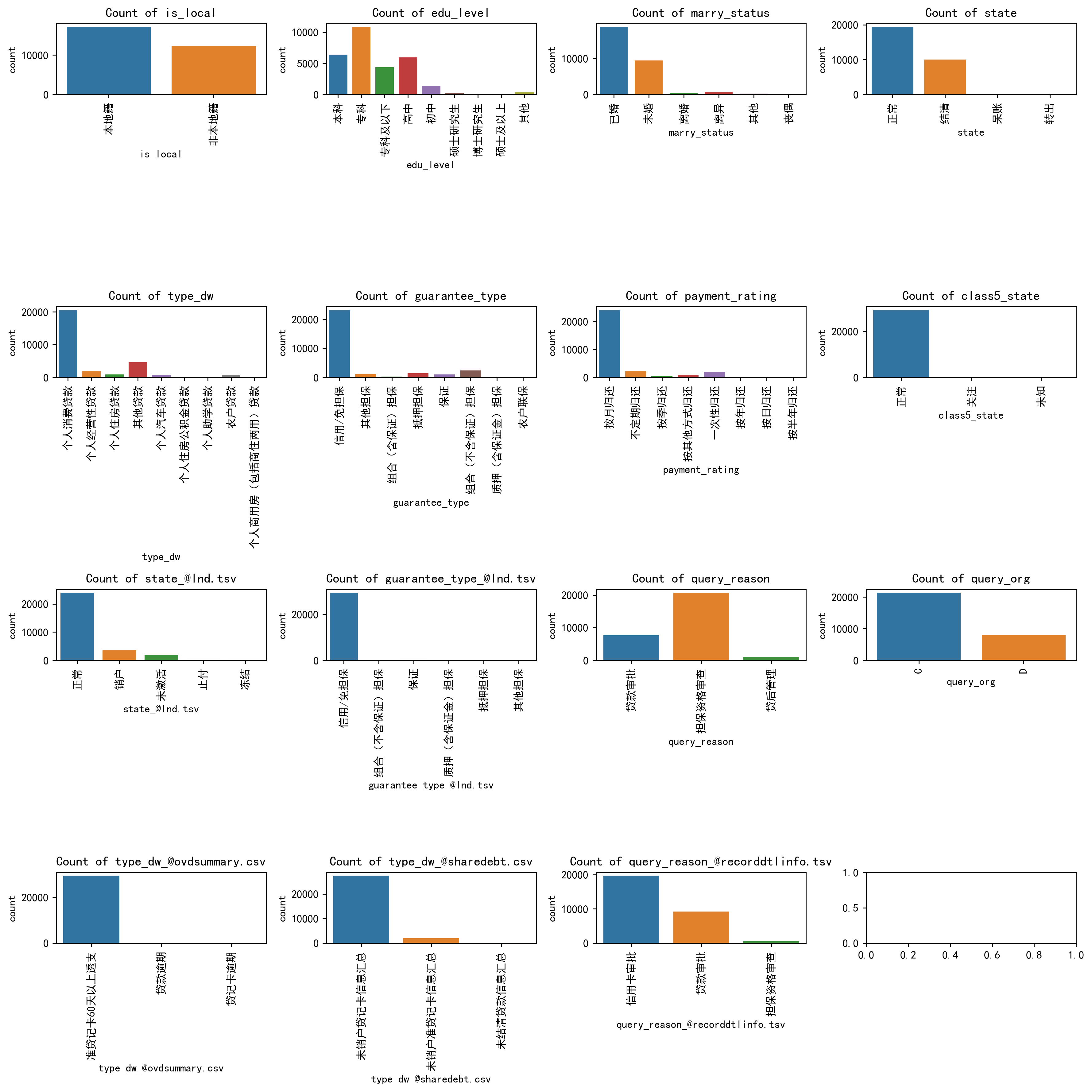

可以很清楚的看到每一個類別變量的哪些類別比較多的類別分布。

數值變量可視化

#畫密度圖，
num_columns = df.select_dtypes(include=['int64', 'float64']).columns.tolist() # 列表頭
dis_cols = 4                   #一行幾個
dis_rows = len(num_columns)
plt.figure(figsize=(3 * dis_cols, 2 * dis_rows),dpi=256)for i in range(len(num_columns)):ax = plt.subplot(dis_rows, dis_cols, i+1)ax = sns.kdeplot(df[num_columns[i]], color="skyblue" ,fill=True)ax.set_xlabel(num_columns[i],fontsize = 14)
plt.tight_layout()
#plt.savefig('訓練測試特征變量核密度圖',formate='png',dpi=500)
plt.show()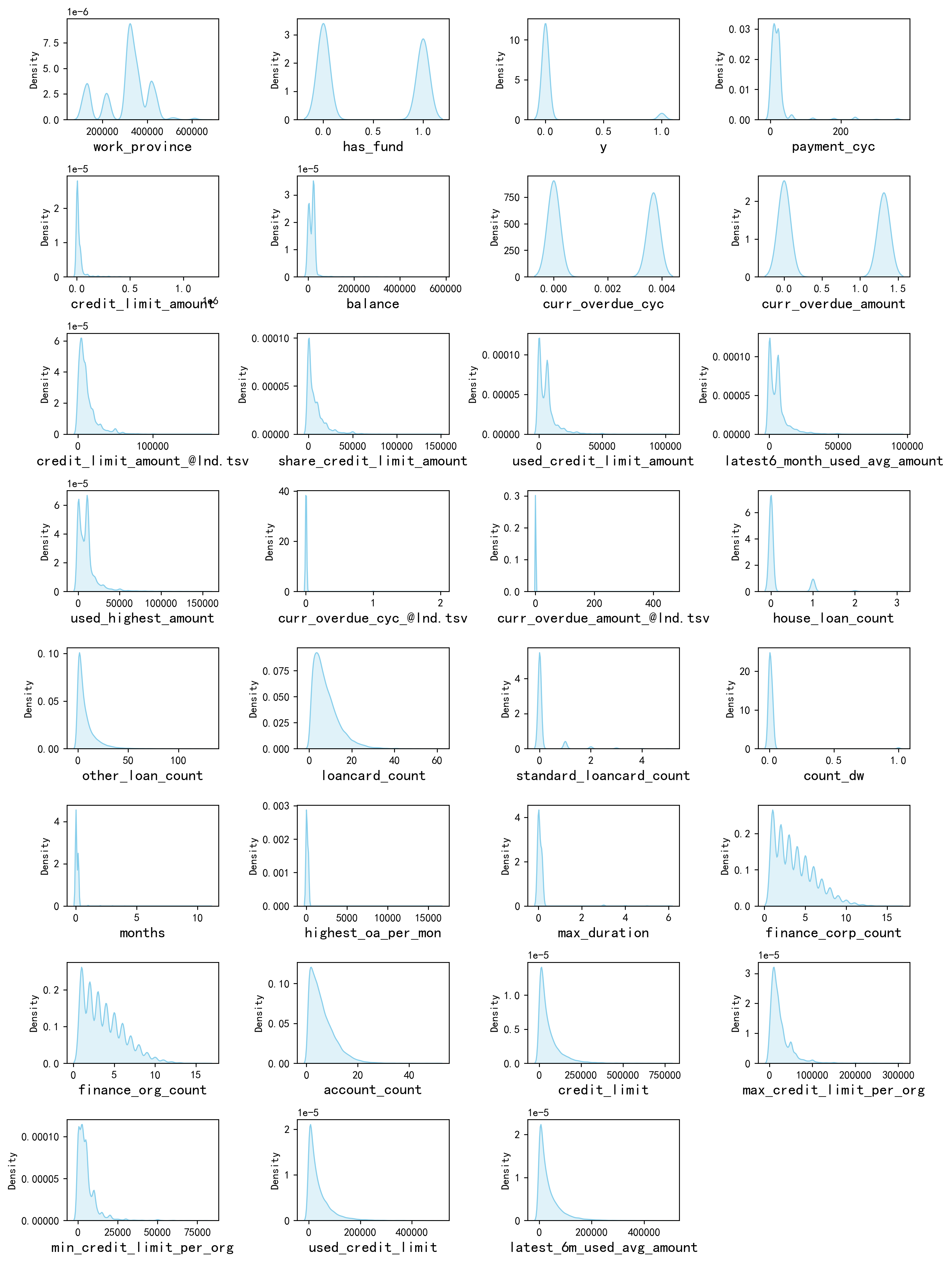

具體的結論就不一個變量一個變量的看了，可以很清楚的看到每一個變量的一些分布的特點。例如他們基本都是右偏分布，也就是說具有一些極大值。

和y進行變量之間的相關性研究

# 將數據按 'edu_level' 和 'y' 進行分組，然后計數
edu_vs_y = df_category.groupby(['edu_level', 'y']).size().unstack()# 將數據按 'marry_status' 和 'y' 進行分組，然后計數
marry_vs_y = df_category.groupby(['marry_status', 'y']).size().unstack()# 創建子圖
fig, axes = plt.subplots(1, 2, figsize=(12, 4), dpi=128)# 繪制第一個子圖的分組條形圖
edu_vs_y.plot(kind='bar', stacked=False, ax=axes[0])
axes[0].set_title('不同教育水平的違約情況')
axes[0].set_xlabel('教育水平')
axes[0].set_ylabel('計數')
axes[0].legend(title='是否違約', loc='upper right')# 繪制第二個子圖的分組條形圖
marry_vs_y.plot(kind='bar', stacked=False, ax=axes[1])
axes[1].set_title('不同婚姻狀態的違約情況')
axes[1].set_xlabel('婚姻狀態')
axes[1].set_ylabel('計數')
axes[1].legend(title='是否違約', loc='upper right')# 調整子圖之間的間距
plt.tight_layout()# 顯示圖形
plt.show()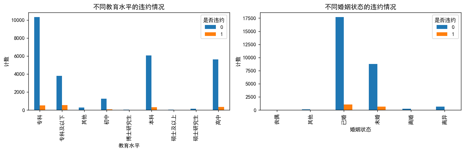

## 看不出明顯的區別

計算相關性系數的熱力圖

corr = plt.subplots(figsize = (18,16),dpi=128)
corr= sns.heatmap(df.corr(method='spearman'),annot=True,square=True)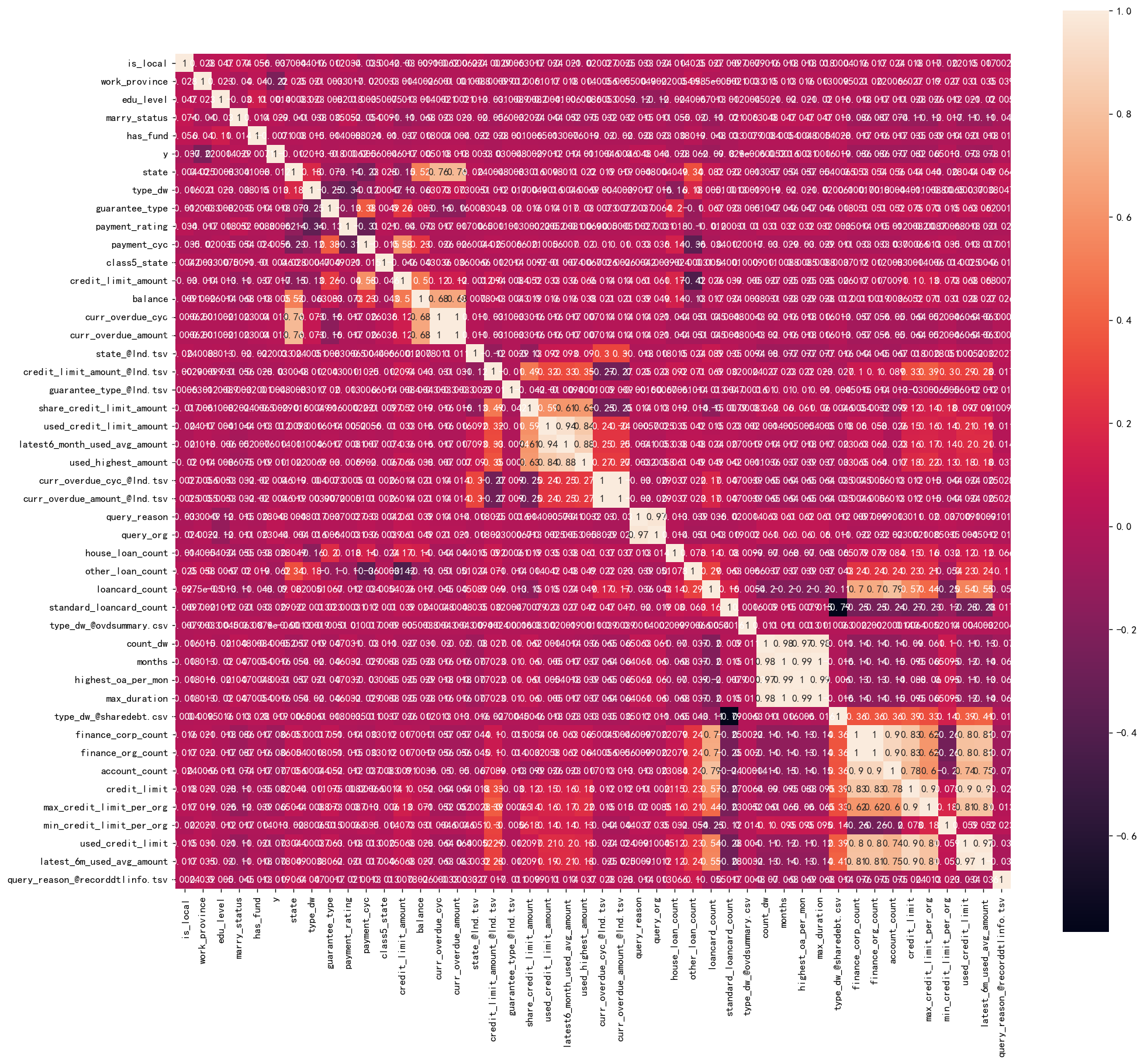

變量有點多，所以說這里就不詳細寫哪些變量和哪些變量之間的相關性比較高了。

---

特征工程

## 前面對數據已經進行了很多預處理了，現在就是要對數據進行進行標準化

#首先取出X和y

X=df.drop('y',axis=1)
y=df['y']

?標準化

# 進行標準化
#數據標準化
from sklearn.preprocessing import StandardScaler
scaler = StandardScaler()
scaler.fit(X)
X_s = scaler.transform(X)
print('標準化后數據形狀：')
print(X_s.shape,y.shape)

---

實驗過程

機器學習——模型選擇

我們首先定義分類問題所使用的評價指標：準確率，精準度，召回率，F1值

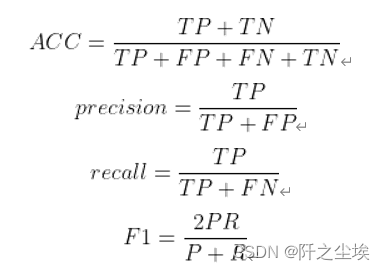
定義評價指標

from sklearn.metrics import confusion_matrix
from sklearn.metrics import classification_report
from sklearn.metrics import cohen_kappa_scoredef evaluation(y_test, y_predict):accuracy=classification_report(y_test, y_predict,output_dict=True)['accuracy']s=classification_report(y_test, y_predict,output_dict=True)['weighted avg']precision=s['precision']recall=s['recall']f1_score=s['f1-score']#kappa=cohen_kappa_score(y_test, y_predict)return accuracy,precision,recall,f1_score #, kappa

?

訓練集測試集劃分

#劃分訓練集和測試集
from sklearn.model_selection import train_test_split
X_train,X_test,y_train,y_test=train_test_split(X_s,y,stratify=y,test_size=0.2,random_state=0)
print(X_train.shape,X_test.shape,y_train.shape,y_test.shape)

### 查看訓練和測試集的y的黑白占比
?

y_train.value_counts(normalize=True)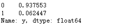

y_test.value_counts(normalize=True)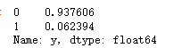

?兩者比例是類似的，不過樣本很不平衡，取值為1的太少了，所以我們要做一點采樣處理。

在處理極度不平衡的分類樣本時，可以考慮以下幾種方法： 欠采樣（Undersampling）：從多數類別中隨機選擇一部分樣本，使得多數類別的樣本數量與少數類別的樣本數量相近。這種方法的優點是簡單快捷，但可能會丟失一些有用信息。

過采樣（Oversampling）：從少數類別中隨機復制一些樣本，使得少數類別的樣本數量與多數類別的樣本數量相近。這種方法的優點是可以充分利用數據集，但可能會導致過擬合。

SMOTE（Synthetic Minority Over-sampling Technique）算法：是一種常用的過采樣方法，它通過對少數類別樣本進行插值生成新的樣本來擴充數據集。這種方法可以有效地避免過擬合問題。

混合采樣（Mixed Sampling）：結合欠采樣和過采樣的優點，既可以減少數據量，又可以充分利用數據集。可以先進行欠采樣，然后再對欠采樣后的數據進行過采樣。

我們首先對樣本少的類別，即逾期類別，取值為1 的進行上采樣。

from imblearn.over_sampling import RandomOverSampler
os=RandomOverSampler(sampling_strategy=0.1)
X_train_ns,y_train_ns=os.fit_resample(X_s,y)
print("The number of classes before fit {}".format(y.value_counts().to_dict()))
print("The number of classes after fit {}".format(y_train_ns.value_counts().to_dict()))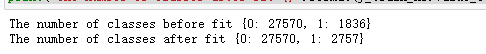

X_train_ns.shape,y_train_ns.shape

再對樣本多的進行下采樣，比例為0.2，即0類數量8成，1類數量2成。雖然也不平衡，但是比剛剛那個好多了。。也能訓練了。

from imblearn.under_sampling import RandomUnderSampler
rus = RandomUnderSampler(sampling_strategy=0.25)
X_resampled, y_resampled = rus.fit_resample(X_train_ns, y_train_ns)
X_train_ns2,y_train_ns2=rus.fit_resample(X_train_ns,y_train_ns)
print("The number of classes before fit {}".format(y_train_ns.value_counts().to_dict()))
print("The number of classes after fit {}".format(y_train_ns2.value_counts().to_dict()))

查看形狀

print(X_train_ns2.shape,y_train_ns2.shape)

##再次重新劃分訓練集和測試集
X_train,X_test,y_train,y_test=train_test_split(X_train_ns2,y_train_ns2,stratify=y_train_ns2,test_size=0.2,random_state=0)
print(X_train.shape,X_test.shape,y_train.shape,y_test.shape)

### 查看訓練和測試集的y的黑白占比
y_train.value_counts(normalize=True)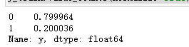

y_test.value_counts(normalize=True)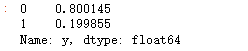

比例大概8:2，比剛剛嚴重不平衡好很多，可以進行機器學習了

---

模型訓練

#導包
from sklearn.linear_model import LogisticRegression
from sklearn.discriminant_analysis import LinearDiscriminantAnalysis
from sklearn.neighbors import KNeighborsClassifier
from sklearn.tree import DecisionTreeClassifier
from sklearn.ensemble import RandomForestClassifier
from sklearn.ensemble import GradientBoostingClassifier
from xgboost.sklearn import XGBClassifier
from lightgbm import LGBMClassifier
from sklearn.svm import SVC
from sklearn.neural_network import MLPClassifier

實例化分類器：

#邏輯回歸
model1 =  LogisticRegression(C=1e10,max_iter=10000)#線性判別分析
model2 = LinearDiscriminantAnalysis()#K近鄰
model3 = KNeighborsClassifier(n_neighbors=10)#決策樹
model4 = DecisionTreeClassifier(random_state=77)#隨機森林
model5= RandomForestClassifier(n_estimators=1000,  max_features='sqrt',random_state=10)#梯度提升
model6 = GradientBoostingClassifier(random_state=123)#極端梯度提升
model7 =  XGBClassifier(objective='binary:logistic',random_state=1)#輕量梯度提升
model8 = LGBMClassifier(objective='binary',random_state=1,verbose=-1)#支持向量機
model9 = SVC(kernel="rbf", random_state=77)#神經網絡
model10 = MLPClassifier(hidden_layer_sizes=(16,8), random_state=77, max_iter=10000)model_list=[model1,model2,model3,model4,model5,model6,model7,model8,model9,model10]
model_name=['邏輯回歸','線性判別','K近鄰','決策樹','隨機森林','梯度提升','極端梯度提升','輕量梯度提升','支持向量機','神經網絡']

訓練和評估

df_eval=pd.DataFrame(columns=['Accuracy','Precision','Recall','F1_score'])
for i in range(10):model_C=model_list[i]name=model_name[i]model_C.fit(X_train, y_train)pred=model_C.predict(X_test)#s=classification_report(y_test, pred)s=evaluation(y_test,pred)df_eval.loc[name,:]=list(s)print(f'{name}模型完成')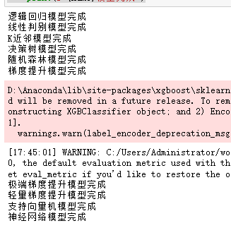

查看評價指標

df_eval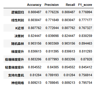

可視化看看

import matplotlib.pyplot as plt 
plt.rcParams['font.sans-serif'] = ['KaiTi']  #中文
plt.rcParams['axes.unicode_minus'] = False   #負號bar_width = 0.4
colors=['c', 'b', 'g', 'tomato', 'm', 'y', 'lime', 'k','orange','pink','grey','tan']
fig, ax = plt.subplots(2,2,figsize=(10,8),dpi=128)
for i,col in enumerate(df_eval.columns):n=int(str('22')+str(i+1))plt.subplot(n)df_col=df_eval[col]m =np.arange(len(df_col))plt.bar(x=m,height=df_col.to_numpy(),width=bar_width,color=colors)#plt.xlabel('Methods',fontsize=12)names=df_col.indexplt.xticks(range(len(df_col)),names,fontsize=10)plt.xticks(rotation=40)plt.ylabel(col,fontsize=14)plt.tight_layout()
#plt.savefig('柱狀圖.jpg',dpi=512)
plt.show()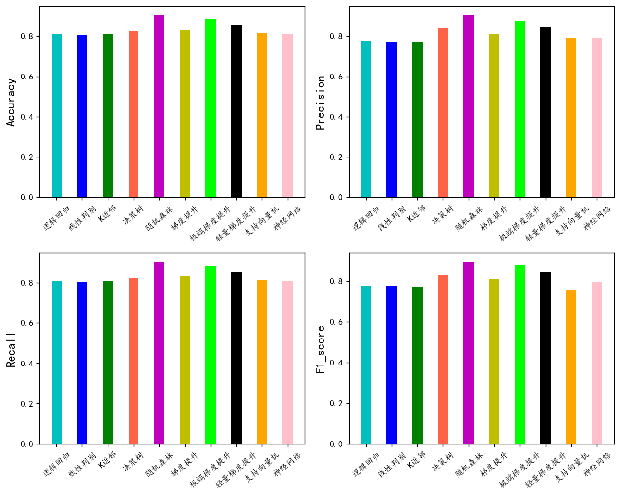

可以看到隨機森林模型效果最好，我們選擇他作為最終模型

超參數搜索

簡單網格化定義幾個超參數，搜索一下。對模型的效果進行一定的優化。

水系森林超凡樹不太多，我們這里就搜索一下最影響最大的估計器個數吧。

# 網格化搜索最優超參數
from sklearn.model_selection import KFold, train_test_split, GridSearchCV
rf_model = RandomForestClassifier(max_features='sqrt',random_state=10)
param_dict = { 'n_estimators': [100,500,700]}
clf = GridSearchCV(rf_model, param_dict, verbose=1,cv=3)
clf.fit(X_train, y_train)
print(clf.best_score_)
print(clf.best_params_)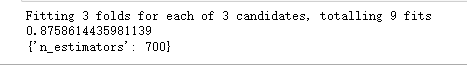

將搜索出來的這個超參數代入模型去訓練

model=RandomForestClassifier( n_estimators=700   , max_features='sqrt',random_state=10)
model.fit(X_train, y_train)
y_pred=model.predict(X_test)
evaluation(y_test,y_pred)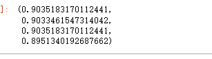

超參數 可以看到整體的準確率精準度召回率f1值，都稍微提高了一些。

?

---

實驗結果

AUC,ROC,KS

信貸場景是一個經典的2分類問題，就是判斷它是不是會違約，從而做出要不要給他貸款的決策。2分類問題就逃不開要計算roc曲線，計算auc值和ks。 用如下的代碼畫出roc曲線跟pr曲線。

from sklearn.metrics import roc_curve, auc, precision_recall_curve
y_pred_proba = model.predict_proba(X_test)[:, 1]
# 計算ROC曲線和AUC值
fpr, tpr, _ = roc_curve(y_test, y_pred_proba)
roc_auc = auc(fpr, tpr)
# 計算PR曲線
precision, recall, _ = precision_recall_curve(y_test, y_pred_proba)# 創建1*2的子圖
plt.figure(figsize=(10, 4),dpi=128)# 繪制ROC曲線
plt.subplot(1, 2, 1)
plt.plot(fpr, tpr, color='tomato', lw=2, label='AUC = %0.2f' % roc_auc)
plt.plot([0, 1], [0, 1], color='k', lw=1, linestyle='--')
plt.xlim([0.0, 1.0]) ;  plt.ylim([0.0, 1.05])
plt.xlabel('False Positive Rate')  ;  plt.ylabel('True Positive Rate')
plt.title('Receiver Operating Characteristic (ROC) Curve')
plt.legend(loc="lower right")# 繪制PR曲線
plt.subplot(1, 2, 2)
plt.plot(recall, precision, color='skyblue', lw=2)
plt.xlim([0.0, 1.0])  ;  plt.ylim([0.0, 1.05])
plt.xlabel('Recall')  ;  plt.ylabel('Precision')
plt.title('Precision-Recall (PR) Curve')# 顯示圖像
plt.tight_layout()
plt.show()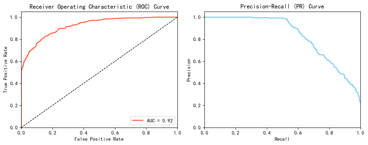

很漂亮的曲線，效果很好，不過也可能是上采樣和下采樣導致的有些樣本重復。

畫KS圖：

import scikitplot as skplt
skplt.metrics.plot_ks_statistic(y_test,model.predict_proba(X_test))
plt.show()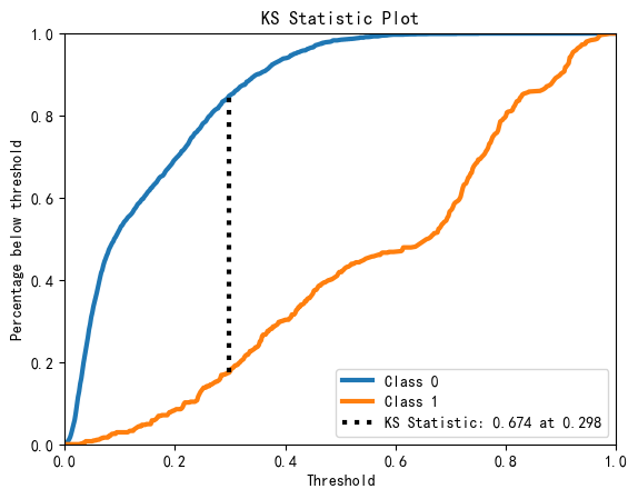

模型的AUC0.92, KS0.674，說明模型效果很好，對好壞客戶有很強的區分能力

進一步的去觀察他每個預測的概率區間里面有多少個樣本，多少個好樣本，壞樣本，壞樣本的比例有多少，它的提升度有多少，累積的這個壞樣本的百分比有多少。

自定義函數

def calculate_pred_proba_bin(true_labels,predictions, bins=10):# 創建分箱區間bin_edges = np.linspace(0, 1, bins + 1)# 分箱bin_labels = [f"{bin_edges[i]:.2f}-{bin_edges[i+1]:.2f}" for i in range(len(bin_edges)-1)]bin_indices = np.digitize(predictions, bin_edges, right=False) - 1# 創建數據框df = pd.DataFrame({ 'bin': [bin_labels[i] for i in bin_indices], 'label': true_labels })# 統計各個分箱的總數、類別為0和1的樣本數result = df.groupby('bin')['label'].agg(total='count',count_0=lambda x: (x == 0).sum(),count_1=lambda x: (x == 1).sum()).reset_index()# 計算壞樣本率和壞樣本在所有壞樣本中的比例total_bad_samples = result['count_1'].sum()result['bad_rate'] = result['count_1'] / result['total']result['bad_percent'] = result['count_1'] / total_bad_samples#result=result.sort_values('bin',ascending=False)result['lift']=result['bad_rate']/(total_bad_samples/result['total'].sum())result['cumulative_bad_percent'] = result['bad_percent'][::-1].cumsum()[::-1]return result.style.bar(color='skyblue').format(subset=['bad_rate','bad_percent','lift','cumulative_bad_percent'], precision=4)def scorecardpy_display_bin(bins_info):df_list = []for col, bin_data in bins_info.items():df = pd.DataFrame(bin_data)df_list.append(df)result_df = pd.concat(df_list, ignore_index=True)# 增加 lift 列total_bad = result_df['bad'].sum()   ;   total_count = result_df['count'].sum()overall_bad_rate = total_bad / total_countresult_df['lift'] = result_df['badprob'] / overall_bad_rateresult_df=result_df.sort_values(['total_iv','variable'],ascending=False).set_index(['variable','total_iv','bin'])[['count_distr','count','good','bad','badprob','lift','bin_iv','woe']]return  result_df.style.format(subset=['count','good','bad'], precision=0).format(subset=['count_distr', 'bad','lift','badprob','woe','bin_iv'], precision=4).bar(subset=['badprob','bin_iv','lift'], color=['#d65f5f', '#5fba7d'])

calculate_pred_proba_bin(y_test,y_pred_proba, bins=20)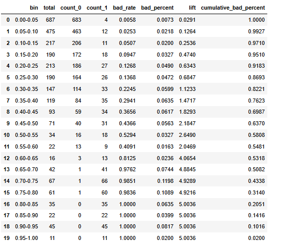

基本上隨著模型的概率越來越高，模型預測正確的把握越來越大，其提升度也就是每一箱的這個黑樣本的比例也是越來越高的。說明模型其性能沒有什么太多的問題。

如果要進行使用的話建議是可以模型預測概率為0.6區間以上的全部拒絕掉，可以過濾到50%的黑樣本，0.15到0.5之間的樣本再進行一次審查，0.15以下的貸款可以接受.