應用cnn對kaggle上的圖像數據集進行練習
數據集地址:Cat and Dog
import torch
import torch.nn as nn
import torch.optim as optim
from torchvision import datasets, transforms
from torch.utils.data import DataLoader
import matplotlib.pyplot as plt
import numpy as np
import matplotlib.pyplot as plt
from PIL import Image
import torch.optim as optim# 設置隨機種子確保結果可復現
# 在深度學習中,隨機種子可以讓每次運行代碼時,模型初始化參數、數據打亂等隨機操作保持一致,方便調試和對比實驗結果
torch.manual_seed(42)
np.random.seed(42)# 設置中文字體支持
plt.rcParams["font.family"] = ["SimHei"]
plt.rcParams['axes.unicode_minus'] = False  # 解決負號顯示問題# 檢查GPU是否可用
device = torch.device("cuda" if torch.cuda.is_available() else "cpu")
print(f"使用設備: {device}")
?數據預處理
# 1. 數據預處理
# 訓練集:使用多種數據增強方法提高模型泛化能力
train_transform = transforms.Compose([# 調整圖像大小為224x224transforms.Resize((224, 224)),# 隨機水平翻轉圖像(概率0.5)transforms.RandomHorizontalFlip(),# 隨機顏色抖動:亮度、對比度、飽和度和色調隨機變化transforms.ColorJitter(brightness=0.2, contrast=0.2, saturation=0.2, hue=0.1),# 隨機旋轉圖像(最大角度15度)transforms.RandomRotation(15),# 將PIL圖像或numpy數組轉換為張量transforms.ToTensor(),# 標準化處理:每個通道的均值和標準差,使數據分布更合理transforms.Normalize((0.4867, 0.4527, 0.4135), (0.2600, 0.2519, 0.2547))
])# 測試集:僅進行必要的標準化,保持數據原始特性,標準化不損失數據信息,可還原
test_transform = transforms.Compose([transforms.Resize((224, 224)),  # 調整圖像大小為224x224transforms.ToTensor(),transforms.Normalize((0.4867, 0.4527, 0.4135), (0.2600, 0.2519, 0.2547))
])# 2. 加載數據集
train_dataset = datasets.ImageFolder(root='./test_set',  # 訓練集圖像所在的根目錄transform=train_transform  # 使用增強后的預處理
)test_dataset = datasets.ImageFolder(root='./training_set',  # 測試集圖像所在的根目錄transform=test_transform  # 測試集不使用增強
)# 3. 創建數據加載器
batch_size = 64
train_loader = DataLoader(train_dataset, batch_size=batch_size, shuffle=True)
test_loader = DataLoader(test_dataset, batch_size=batch_size, shuffle=False)
CNN模型的定義?
# 4. 定義CNN模型
class CNN(nn.Module):def __init__(self):super(CNN, self).__init__()  # 繼承父類初始化# ---------------------- 第一個卷積塊 ----------------------# 卷積層1:輸入3通道(RGB),輸出32個特征圖,卷積核3x3,邊緣填充1像素self.conv1 = nn.Conv2d(in_channels=3,       # 輸入通道數(圖像的RGB通道)out_channels=32,     # 輸出通道數(生成32個新特征圖)kernel_size=3,       # 卷積核尺寸(3x3像素)padding=1            # 邊緣填充1像素,保持輸出尺寸與輸入相同)# 批量歸一化層:對32個輸出通道進行歸一化,加速訓練self.bn1 = nn.BatchNorm2d(num_features=32)# ReLU激活函數:引入非線性,公式:max(0, x)self.relu1 = nn.ReLU()# 最大池化層:窗口2x2,步長2,特征圖尺寸減半(224x224→112x112)self.pool1 = nn.MaxPool2d(kernel_size=2, stride=2)  # stride默認等于kernel_size# ---------------------- 第二個卷積塊 ----------------------# 卷積層2:輸入32通道(來自conv1的輸出),輸出64通道self.conv2 = nn.Conv2d(in_channels=32,      # 輸入通道數(前一層的輸出通道數)out_channels=64,     # 輸出通道數(特征圖數量翻倍)kernel_size=3,       # 卷積核尺寸不變padding=1            # 保持尺寸:112x112→112x112(卷積后)→56x56(池化后))self.bn2 = nn.BatchNorm2d(num_features=64)self.relu2 = nn.ReLU()self.pool2 = nn.MaxPool2d(kernel_size=2)  # 尺寸減半:112x112→56x56# ---------------------- 第三個卷積塊 ----------------------# 卷積層3:輸入64通道,輸出128通道self.conv3 = nn.Conv2d(in_channels=64,      # 輸入通道數(前一層的輸出通道數)out_channels=128,    # 輸出通道數(特征圖數量再次翻倍)kernel_size=3,padding=1            # 保持尺寸:56x56→56x56(卷積后)→28x28(池化后))self.bn3 = nn.BatchNorm2d(num_features=128)self.relu3 = nn.ReLU()  # 復用激活函數對象(節省內存)self.pool3 = nn.MaxPool2d(kernel_size=2)  # 尺寸減半:56x56→28x28# ---------------------- 全連接層(分類器) ----------------------# 計算展平后的特征維度:128通道 × 28x28尺寸 = 128×784=100352維self.fc1 = nn.Linear(in_features=128 * 28 * 28,  # 輸入維度(卷積層輸出的特征數)out_features=512          # 輸出維度(隱藏層神經元數))# Dropout層:訓練時隨機丟棄50%神經元,防止過擬合self.dropout = nn.Dropout(p=0.5)# 輸出層:將512維特征映射到2個類別(類別數)self.fc2 = nn.Linear(in_features=512, out_features=2)def forward(self, x):# 輸入尺寸:[batch_size, 3, 224, 224](batch_size=批量大小,3=通道數,224x224=圖像尺寸)# ---------- 卷積塊1處理 ----------x = self.conv1(x)       # 卷積后尺寸:[batch_size, 32, 224, 224](padding=1保持尺寸)x = self.bn1(x)         # 批量歸一化,不改變尺寸x = self.relu1(x)       # 激活函數,不改變尺寸x = self.pool1(x)       # 池化后尺寸:[batch_size, 32, 112, 112](224→112是因為池化窗口2x2)# ---------- 卷積塊2處理 ----------x = self.conv2(x)       # 卷積后尺寸:[batch_size, 64, 112, 112](padding=1保持尺寸)x = self.bn2(x)x = self.relu2(x)x = self.pool2(x)       # 池化后尺寸:[batch_size, 64, 56, 56]# ---------- 卷積塊3處理 ----------x = self.conv3(x)       # 卷積后尺寸:[batch_size, 128, 56, 56](padding=1保持尺寸)x = self.bn3(x)x = self.relu3(x)x = self.pool3(x)       # 池化后尺寸:[batch_size, 128, 28, 28]# ---------- 展平與全連接層 ----------# 將多維特征圖展平為一維向量:[batch_size, 128*28*28] = [batch_size, 100352]x = x.view(-1, 128 * 28 * 28)  # -1自動計算批量維度,保持批量大小不變x = self.fc1(x)           # 全連接層:100352→512,尺寸變為[batch_size, 512]x = self.relu3(x)         # 激活函數(復用relu3,與卷積塊3共用)x = self.dropout(x)       # Dropout隨機丟棄神經元,不改變尺寸x = self.fc2(x)           # 全連接層:512→2,尺寸變為[batch_size, 2](未激活,直接輸出logits)return x  # 輸出未經過Softmax的logits,適用于交叉熵損失函數# 初始化模型
model = CNN()
model = model.to(device)  # 將模型移至GPU(如果可用)
criterion = nn.CrossEntropyLoss() # 交叉熵損失函數
optimizer = optim.Adam(model.parameters(), lr=0.001) # Adam優化器# 引入學習率調度器,在訓練過程中動態調整學習率--訓練初期使用較大的 LR 快速降低損失,訓練后期使用較小的 LR 更精細地逼近全局最優解。
# 在每個 epoch 結束后,需要手動調用調度器來更新學習率,可以在訓練過程中調用 scheduler.step()
scheduler = optim.lr_scheduler.ReduceLROnPlateau(optimizer, # 指定要控制的優化器(這里是Adam)mode='min', # 監測的指標是"最小化"(如損失函數)patience=3, # 如果連續3個epoch指標沒有改善,才降低LRfactor=0.5 # 降低LR的比例(新LR = 舊LR × 0.5)?訓練模型
# 5. 訓練模型(記錄每個 iteration 的損失)
def train(model, train_loader, test_loader, criterion, optimizer, scheduler, device, epochs):model.train()  # 設置為訓練模式# 記錄每個 iteration 的損失all_iter_losses = []  # 存儲所有 batch 的損失iter_indices = []     # 存儲 iteration 序號# 記錄每個 epoch 的準確率和損失train_acc_history = []test_acc_history = []train_loss_history = []test_loss_history = []for epoch in range(epochs):running_loss = 0.0correct = 0total = 0for batch_idx, (data, target) in enumerate(train_loader):data, target = data.to(device), target.to(device)  # 移至GPUoptimizer.zero_grad()  # 梯度清零output = model(data)  # 前向傳播loss = criterion(output, target)  # 計算損失loss.backward()  # 反向傳播optimizer.step()  # 更新參數# 記錄當前 iteration 的損失iter_loss = loss.item()all_iter_losses.append(iter_loss)iter_indices.append(epoch * len(train_loader) + batch_idx + 1)# 統計準確率和損失running_loss += iter_loss_, predicted = output.max(1)total += target.size(0)correct += predicted.eq(target).sum().item()# 每100個批次打印一次訓練信息if (batch_idx + 1) % 100 == 0:print(f'Epoch: {epoch+1}/{epochs} | Batch: {batch_idx+1}/{len(train_loader)} 'f'| 單Batch損失: {iter_loss:.4f} | 累計平均損失: {running_loss/(batch_idx+1):.4f}')# 計算當前epoch的平均訓練損失和準確率epoch_train_loss = running_loss / len(train_loader)epoch_train_acc = 100. * correct / totaltrain_acc_history.append(epoch_train_acc)train_loss_history.append(epoch_train_loss)# 測試階段model.eval()  # 設置為評估模式test_loss = 0correct_test = 0total_test = 0with torch.no_grad():for data, target in test_loader:data, target = data.to(device), target.to(device)output = model(data)test_loss += criterion(output, target).item()_, predicted = output.max(1)total_test += target.size(0)correct_test += predicted.eq(target).sum().item()epoch_test_loss = test_loss / len(test_loader)epoch_test_acc = 100. * correct_test / total_testtest_acc_history.append(epoch_test_acc)test_loss_history.append(epoch_test_loss)# 更新學習率調度器scheduler.step(epoch_test_loss)print(f'Epoch {epoch+1}/{epochs} 完成 | 訓練準確率: {epoch_train_acc:.2f}% | 測試準確率: {epoch_test_acc:.2f}%')# 繪制所有 iteration 的損失曲線plot_iter_losses(all_iter_losses, iter_indices)# 繪制每個 epoch 的準確率和損失曲線plot_epoch_metrics(train_acc_history, test_acc_history, train_loss_history, test_loss_history)return epoch_test_acc  # 返回最終測試準確率# 6. 繪制每個 iteration 的損失曲線
def plot_iter_losses(losses, indices):plt.figure(figsize=(10, 4))plt.plot(indices, losses, 'b-', alpha=0.7, label='Iteration Loss')plt.xlabel('Iteration(Batch序號)')plt.ylabel('損失值')plt.title('每個 Iteration 的訓練損失')plt.legend()plt.grid(True)plt.tight_layout()plt.show()# 7. 繪制每個 epoch 的準確率和損失曲線
def plot_epoch_metrics(train_acc, test_acc, train_loss, test_loss):epochs = range(1, len(train_acc) + 1)plt.figure(figsize=(12, 4))# 繪制準確率曲線plt.subplot(1, 2, 1)plt.plot(epochs, train_acc, 'b-', label='訓練準確率')plt.plot(epochs, test_acc, 'r-', label='測試準確率')plt.xlabel('Epoch')plt.ylabel('準確率 (%)')plt.title('訓練和測試準確率')plt.legend()plt.grid(True)# 繪制損失曲線plt.subplot(1, 2, 2)plt.plot(epochs, train_loss, 'b-', label='訓練損失')plt.plot(epochs, test_loss, 'r-', label='測試損失')plt.xlabel('Epoch')plt.ylabel('損失值')plt.title('訓練和測試損失')plt.legend()plt.grid(True)plt.tight_layout()plt.show()# 8. 執行訓練和測試
epochs = 5  # 增加訓練輪次以獲得更好效果
print("開始使用CNN訓練模型...")
final_accuracy = train(model, train_loader, test_loader, criterion, optimizer, scheduler, device, epochs)
print(f"訓練完成!最終測試準確率: {final_accuracy:.2f}%")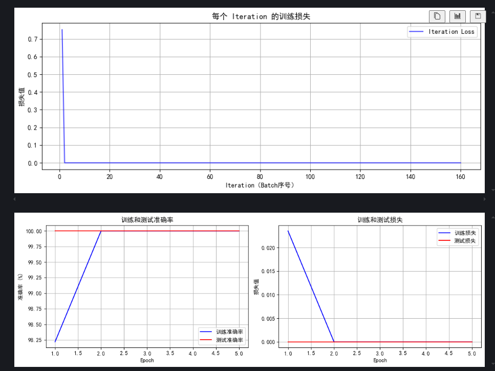
Grad-CAM實現
# Grad-CAM實現
class GradCAM:def __init__(self, model, target_layer):self.model = modelself.target_layer = target_layerself.gradients = Noneself.activations = None# 注冊鉤子,用于獲取目標層的前向傳播輸出和反向傳播梯度self.register_hooks()def register_hooks(self):# 前向鉤子函數,在目標層前向傳播后被調用,保存目標層的輸出(激活值)def forward_hook(module, input, output):self.activations = output.detach()# 反向鉤子函數,在目標層反向傳播后被調用,保存目標層的梯度def backward_hook(module, grad_input, grad_output):self.gradients = grad_output[0].detach()# 在目標層注冊前向鉤子和反向鉤子self.target_layer.register_forward_hook(forward_hook)self.target_layer.register_backward_hook(backward_hook)def generate_cam(self, input_image, target_class=None):# 前向傳播,得到模型輸出model_output = self.model(input_image)if target_class is None:# 如果未指定目標類別,則取模型預測概率最大的類別作為目標類別target_class = torch.argmax(model_output, dim=1).item()# 清除模型梯度,避免之前的梯度影響self.model.zero_grad()# 反向傳播,構造one-hot向量,使得目標類別對應的梯度為1,其余為0,然后進行反向傳播計算梯度one_hot = torch.zeros_like(model_output)one_hot[0, target_class] = 1model_output.backward(gradient=one_hot)# 獲取之前保存的目標層的梯度和激活值gradients = self.gradientsactivations = self.activations# 對梯度進行全局平均池化,得到每個通道的權重,用于衡量每個通道的重要性weights = torch.mean(gradients, dim=(2, 3), keepdim=True)# 加權激活映射,將權重與激活值相乘并求和,得到類激活映射的初步結果cam = torch.sum(weights * activations, dim=1, keepdim=True)# ReLU激活,只保留對目標類別有正貢獻的區域,去除負貢獻的影響cam = F.relu(cam)# 調整大小并歸一化,將類激活映射調整為與輸入圖像相同的尺寸(32x32),并歸一化到[0, 1]范圍cam = F.interpolate(cam, size=(32, 32), mode='bilinear', align_corners=False)cam = cam - cam.min()cam = cam / cam.max() if cam.max() > 0 else camreturn cam.cpu().squeeze().numpy(), target_class
熱力圖?
import warnings
warnings.filterwarnings("ignore")
import matplotlib.pyplot as plt
# 設置中文字體支持
plt.rcParams["font.family"] = ["SimHei"]
plt.rcParams['axes.unicode_minus'] = False  # 解決負號顯示問題
# 選擇一個隨機圖像
idx = 50  # 選擇測試集中的第101張圖片 (索引從0開始)
image, label = test_dataset[idx]# 轉換圖像以便可視化
def tensor_to_np(tensor):img = tensor.cpu().numpy().transpose(1, 2, 0)mean = np.array([0.4867, 0.4527, 0.4135])std = np.array([0.2600, 0.2519, 0.2547])img = std * img + meanimg = np.clip(img, 0, 1)return img# 添加批次維度并移動到設備
input_tensor = image.unsqueeze(0).to(device)# 初始化Grad-CAM(選擇最后一個卷積層)
grad_cam = GradCAM(model, model.conv3)# 生成熱力圖
heatmap, pred_class = grad_cam.generate_cam(input_tensor)# 可視化
plt.figure(figsize=(12, 4))# 原始圖像
plt.subplot(1, 3, 1)
plt.imshow(tensor_to_np(image))
plt.title(f"原始圖像")
plt.axis('off')# 熱力圖
plt.subplot(1, 3, 2)
plt.imshow(heatmap, cmap='jet')
plt.title(f"Grad-CAM熱力圖")
plt.axis('off')plt.tight_layout()
plt.savefig('grad_cam_result.png')
plt.show()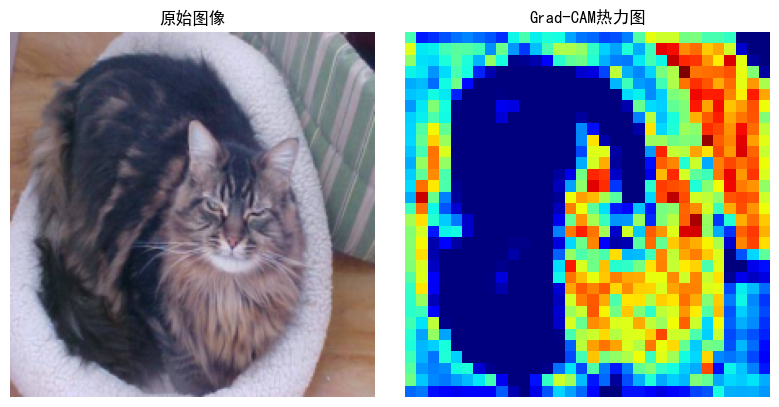
@浙大疏錦行

)


:網絡組成與三種交換方式全解析)
![[總結]前端性能指標分析、性能監控與分析、Lighthouse性能評分分析](http://pic.xiahunao.cn/[總結]前端性能指標分析、性能監控與分析、Lighthouse性能評分分析)


