Attention是Transformer的核心,本系列先通過介紹Attention來學習Transformer。本文先介紹簡單版的Attention。
在Attention出現之前,通常使用recurrent neural networds (RNNs)來處理長序列數據。模型架構上,又通常使用encoder-decoder的結構。
以機器翻譯為例,當輸入文本序列一個一個進入encoder時,encoder也在一步一步地更新它的hidden state(即隱藏層的值)。通過這種方式,encoder在最后一次更新完hidden state后,盡可能多地把整個輸入文本序列的含義捕捉存儲到最終的hidden state中。decoder以encoder的最終hidden state作為輸入,一次一個字地開始翻譯。同樣,decoder也是一步一步地更新它的hidden state,每一次更新后的hidden state都包含了預測下一個字的必要上下文信息。下面的圖就是整個流程:
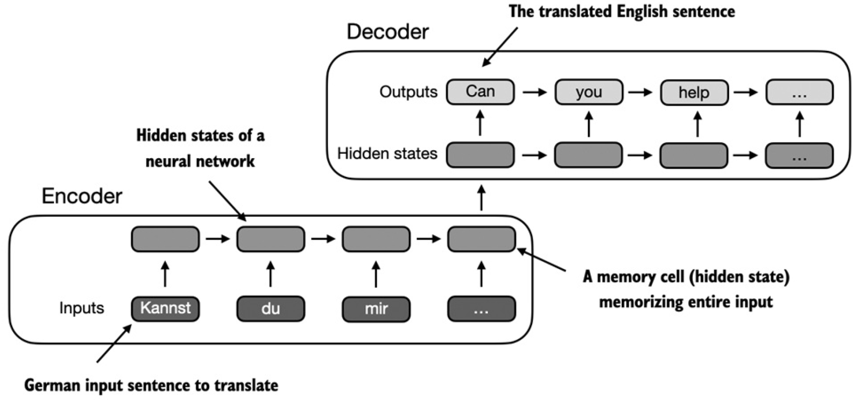
整個流程的關鍵點是encoder將整個文本序列處理成最終的hidden state(memory cell)。decoder以encoder最終的hidden state為輸入,生成輸出。encoder-decoder RNN架構最大的問題和局限性是在decoding階段,RNN無法直接訪問encoder中比較靠前的hidden state。結果decoder只能基于包含了所有相關信息的最終hidden state。當遇到復雜的前后依賴距離跨度大的長句時,這個問題會導致上下文信息的丟失。
Transformer的提出解決了RNN的缺陷并逐漸取代了RNN在NLP領域的位置。而Transformer的核心正是self-attention。self-attention是這樣一套機制,當計算一個序列的表示時,它允許序列中每個位置上的元素去關注序列中其他位置(包括它本身)的元素。self-attention中的"self"是指這套機制能夠通過比較當前位置元素與其他所有位置元素的相關性來計算出關注度權重(attention weights)。它評估學習了輸入自己本身不同部分之間的聯系和依賴關系。
有了上面的基本概念之后,下面先看一個沒有訓練權重的simple self-attention。
假設現在有一個6個單詞的序列,每個單詞的embedding維度是3。
import torch
inputs = torch.tensor(
[[0.43, 0.15, 0.89], # Your (x^1)
[0.55, 0.87, 0.66], # journey (x^2)
[0.57, 0.85, 0.64], # starts (x^3)
[0.22, 0.58, 0.33], # with (x^4)
[0.77, 0.25, 0.10], # one (x^5)
[0.05, 0.80, 0.55]] # step (x^6)
)
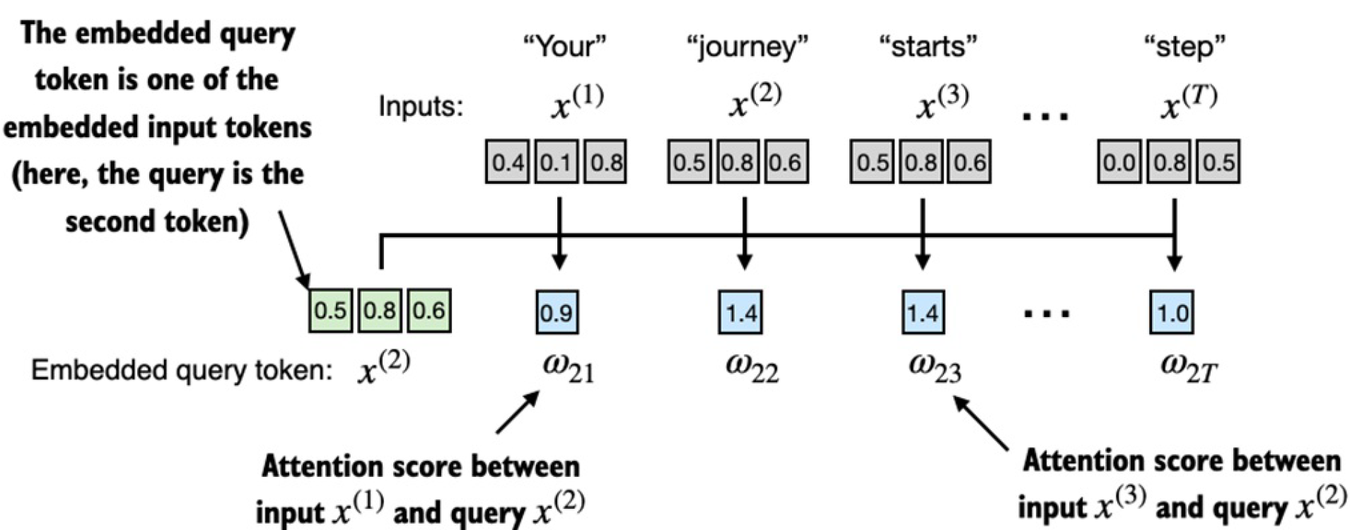
現在我們想要計算第二個單詞跟其他所有單詞的attention weight。首先我們先計算attention score:
query = inputs[1]
attn_scores_2 = torch.empty(inputs.shape[0])
for i, x_i in enumerate(inputs):attn_scores_2[i] = torch.dot(x_i, query)
print(attn_scores_2)
# 輸出:
# tensor([0.9544, 1.4950, 1.4754, 0.8434, 0.7070, 1.0865])
這里我們使用的點乘(dot product)。點乘是將兩個向量element-wise地相乘然后相加。點乘結果越大表明兩個向量越相關。這部分過程如下圖所示:
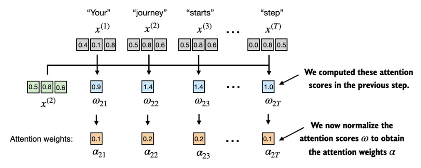
接下來,我們對attention score做歸一化求attention weight。
attn_weights_2_tmp = attn_scores_2 / attn_scores_2.sum()
print("Attention weights:", attn_weights_2_tmp)
print("Sum:", attn_weights_2_tmp.sum())
# 輸出:
# Attention weights: tensor([0.1455, 0.2278, 0.2249, 0.1285, 0.1077, 0.1656])
# Sum: tensor(1.0000)
實際中,主要是用PyTorch自帶的softmax函數來做這個歸一化:
attn_weights_2 = torch.softmax(attn_scores_2, dim=0)
print("Attention weights:", attn_weights_2)
print("Sum:", attn_weights_2.sum())
# 輸出:
# Attention weights: tensor([0.1385, 0.2379, 0.2333, 0.1240, 0.1082, 0.1581])
# Sum: tensor(1.)
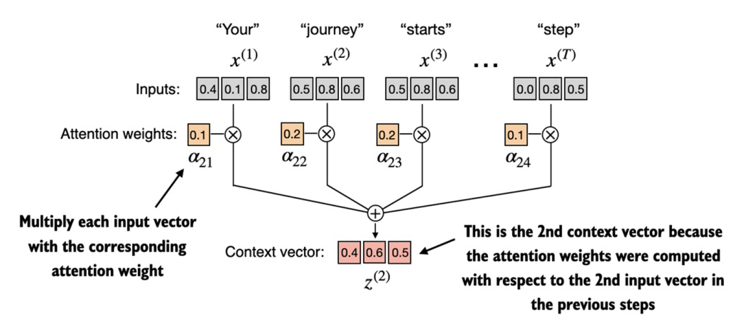
有了attention weight之后,就是最后一步,求第二個單詞的上下文向量。
query = inputs[1] # 2nd input token is the query
context_vec_2 = torch.zeros(query.shape)
for i,x_i in enumerate(inputs):
context_vec_2 += attn_weights_2[i]*x_i
print(context_vec_2)
# 輸出:
# tensor([0.4419, 0.6515, 0.5683])
上面是計算第二個單詞的上下文向量,下面我們一次性地求所有單詞的上下文向量:
# @ 是矩陣乘法,inputs.T 是轉置操作
attn_scores = inputs @ inputs.T
print(attn_scores)
# tensor([[0.9995, 0.9544, 0.9422, 0.4753, 0.4576, 0.6310],
# [0.9544, 1.4950, 1.4754, 0.8434, 0.7070, 1.0865],
# [0.9422, 1.4754, 1.4570, 0.8296, 0.7154, 1.0605],
# [0.4753, 0.8434, 0.8296, 0.4937, 0.3474, 0.6565],
# [0.4576, 0.7070, 0.7154, 0.3474, 0.6654, 0.2935],
# [0.6310, 1.0865, 1.0605, 0.6565, 0.2935, 0.9450]])# 注意在第一維上做softmax
attn_weights = torch.softmax(attn_scores, dim=1)
print(attn_weights)
# 可以看到每一行加起來都是1
# tensor([[0.2098, 0.2006, 0.1981, 0.1242, 0.1220, 0.1452],
# [0.1385, 0.2379, 0.2333, 0.1240, 0.1082, 0.1581],
# [0.1390, 0.2369, 0.2326, 0.1242, 0.1108, 0.1565],
# [0.1435, 0.2074, 0.2046, 0.1462, 0.1263, 0.1720],
# [0.1526, 0.1958, 0.1975, 0.1367, 0.1879, 0.1295],
# [0.1385, 0.2184, 0.2128, 0.1420, 0.0988, 0.1896]])all_context_vecs = attn_weights @ inputs
print(all_context_vecs)
# tensor([[0.4421, 0.5931, 0.5790],
# [0.4419, 0.6515, 0.5683],
# [0.4431, 0.6496, 0.5671],
# [0.4304, 0.6298, 0.5510],
# [0.4671, 0.5910, 0.5266],
# [0.4177, 0.6503, 0.5645]])
本文介紹了一種簡單版的self-attention,即通過兩個詞向量點乘求出兩個詞向量的相關性。下一篇文章,我們將介紹帶可訓練參數的self-attention。
參考資料:
《Build a Large Language Model from scratch》


)


)

)

)