Title

題目

AI-based association analysis for medical imaging using latent-spacegeometric confounder correction

基于人工智能的醫學影像關聯分析：利用潛在空間幾何混雜因素校正法?

01

文獻速遞介紹

人工智能（AI）已成為各個領域的強大助力，這在很大程度上歸功于它能夠在高維數據集中識別出具有判別性的模式。這種能力在醫學影像分析領域尤其有用，事實證明，人工智能技術在診斷和預后預測任務中取得了成功（沈等人，2017）。然而，人工智能在基于醫學影像的流行病學關聯分析中的應用面臨著一些挑戰。這些挑戰包括從人工智能生成的結果中得出具有臨床或流行病學重要意義的見解，與傳統統計方法相比（穆格利等人，2017；豪等人，2019；羅什丘普金等人，2016b），這項任務已被證明頗具難度（宋和霍珀，2023；達菲等人，2022）。這主要有兩個原因：一是人工智能模型中非線性建模的可視化較為復雜，也就是所謂的“黑箱”問題；二是缺乏對混雜變量的控制。這些障礙凸顯了在醫學應用中需要更具可解釋性且無混雜因素的人工智能模型。 1.1 相關工作 1.1.1 混雜因素 混雜因素是在關聯分析中同時影響自變量和因變量的變量（彼得斯等人，2017；斯圖爾特，2022）。因此，它可能會錯誤地產生、放大或減弱這些變量之間的關聯。例如，在一項研究疾病嚴重程度（自變量）與患者康復時間（因變量）之間關聯的研究中，患者患病前的整體健康狀況可能是一個混雜因素，因為疾病嚴重程度和康復時間都可能受到患者整體健康狀況的影響。所以，如果不控制這個混雜因素，預測康復時間的人工智能模型可能會在不經意間將與整體健康狀況相關的特征納入考慮。而這些特征反過來又會混淆結果，掩蓋僅由疾病嚴重程度對康復時間的影響。 人工智能中的偏差通常源于選擇偏差或數據不平衡等問題（李等人，2021；金等人，2021；李和瓦斯科塞洛斯，2019）。當用于訓練模型的數據不能代表更廣泛的人群時，就會出現這種情況，從而導致有偏差的結果和較差的性能。在關于偏差的研究中，研究人員通常假設訓練數據有偏差而測試數據無偏差。他們提出了旨在提高對測試數據預測性能的方法；與選擇偏差或數據不平衡不同，混雜因素通常存在于現實場景中，無法通過重新選擇或重新采樣數據輕易消除。因此，在混雜因素的背景下，研究人員通常假設混雜因素同時存在于訓練數據和測試數據中。其目的是檢測在消除混雜效應后，因變量和自變量之間是否仍然存在關聯。 盡管在經典的流行病學研究中，這個混雜問題及其解決方案已經得到了很好的確立（斯圖爾特，2022；沃伊諾夫和巴本科，2020；普爾霍辛霍利等人，2012），但人工智能領域在糾正混雜因素方面提供的方法有限。此外，在存在多個混雜因素的情況下，這個問題會更加嚴重，這使得開發無混雜因素的人工智能模型變得至關重要。 1.1.2 人工智能中的混雜因素控制：醫學影像面臨的挑戰 在人工智能領域，與混雜因素控制相關的主題有不同的稱謂，如公平表征學習（范等人，2023；路易佐斯等人，2015；克里格等人，2019；劉等人，2021；薩爾漢等人，2020）、去偏表征學習（李等人，2021；金等人，2021）、通用表征學習（李等人，2021）或不變特征學習（謝等人，2017；阿庫扎瓦等人，2020）。這些方法主要側重于從與特定屬性（即學習目標）相關的輸入數據中學習表征，同時保持與敏感屬性（即混雜因素）無關。特別是當敏感屬性指的是不同的領域來源時，這些方法與領域自適應的研究主題有重疊（范等人，2023；李等人，2021；阿庫扎瓦等人，2020）。 雖然混雜因素的概念源于流行病學，但人工智能領域中提出的大多數方法通常有不同的任務和目標，因此并不能完全解決醫學應用中混雜因素帶來的挑戰（達菲等人，2022；布魯克哈特等人，2010）。（1）混雜因素通常是連續變量（如年齡），然而大多數現有方法是為處理單個二元（如性別）或分類（如種族）混雜因素而設計的（范等人，2023；愛德華茲和斯托基，2015；張等人，2018；路易佐斯等人，2015；李等人，2021；阿庫扎瓦等人，2020；李等人，2021；金等人，2021；薩爾漢等人，2020；澤梅爾等人，2013；沈等人，2022）。這些方法需要將一批訓練樣本劃分為幾個子組（如男性和女性）以消除混雜效應（如性別），這使得它們不適用于更難處理的連續混雜因素；（2）當考慮到醫學研究中普遍存在多個混雜因素時，這個問題變得更加突出，而現有的方法中只有少數（陸等人，2021；文托等人，2022）能夠減輕多個混雜因素的聯合影響；（3）此外，在醫學影像分析中，標簽（包括學習目標和混雜因素）常常缺失，但在無混雜因素模型中利用帶有缺失標簽的圖像數據進行半監督設置的探索仍然有限；（4）現有方法在設計中忽略了圖像特征可視化，這使得在基于圖像的關聯研究中難以解釋或理解研究結果。 認識到這一差距，將注意力轉向專門針對這些挑戰開發方法至關重要。例如，CF Net（趙等人，2020）是一種基于對抗訓練的無混雜因素模型，它用基于統計相關性的對抗損失取代了領域自適應任務中常用的典型交叉熵或均方誤差（MSE）對抗損失。這種調整增強了它對連續混雜因素的支持。另一個值得注意的方法是MDN（陸等人，2021；文托等人，2022），它將線性回歸與插入神經網絡的一個獨特層相結合。這個層專門設計用于過濾掉混雜信息，只允許殘余信號傳遞到后續層。由于線性回歸的固有特性，這種方法支持多個混雜因素。盡管有這些例子，但截至目前，仍然缺乏針對醫學影像中混雜因素帶來的挑戰的人工智能方法。 1.1.3 無混雜因素人工智能模型中可解釋性的挑戰 醫學影像研究領域中大多數與特征解釋相關的技術可以分為兩大類（范德韋爾登等人，2022；范等人，2021）。第一類包括梯度和反向傳播方法，這些方法通常檢查人工智能模型內的梯度或激活情況，創建與輸入圖像相關的顯著圖，并突出顯示對預測結果影響最大的區域。示例方法包括梯度加權類激活映射（Grad-CAM）（塞爾瓦拉朱等人，2017）、SHAP（倫德伯格和李，2017）、深度泰勒（蒙塔馮等人，2017）和逐層反向傳播（巴赫等人，2015）。這些方法可以直接應用于訓練好的無混雜因素模型。例如，CF-Net（趙等人，2020）使用Grad-CAM生成顯著圖，比較有無混雜因素控制時的結果。 第二類方法，如研究中所引用的（劉等人，2021；巴拉克里希南等人，2021；希金斯等人，2016；斯通等人，2017；趙等人，2019），通常涉及定制內置生成模型來操縱潛在空間。這種操縱能夠重建一系列顯示與目標屬性（如年齡）相關的圖像變形的圖像（趙等人，2019）。典型的例子是β-VAE（希金斯等人，2016）和infoGAN（陳等人，2016）。與顯著圖不同，這些重建圖像提供了更豐富的語義信息（趙等人，2019），從而增強了對已建立關聯的理解。然而，這些方法的可解釋性是內在的，不能轉移到其他模型。 這種局限性需要開發配備有混雜因素控制功能的新生成模型。然而，事實證明這項任務具有挑戰性。從潛在空間中去除與混雜因素相關的信息，這是許多無混雜因素模型中的常見方法（愛德華茲和斯托基，2015；謝等人，2017；張等人，2018；趙等人，2020；路易佐斯等人，2015；阿萊米等人，2016；克里格等人，2019；陸等人，2021；文托等人，2022；沈等人，2022），可能會對圖像重建質量產生不利影響（劉等人，2021）。這個問題源于兩個優化目標之間的矛盾：圖像重建旨在在潛在空間中保留盡可能多的信息，例如大腦圖像重建中的年齡細節，而混雜因素緩解旨在去除所有與混雜因素相關的信息。在涉及多個混雜因素的情況下，這種矛盾變得更加明顯。 1.2 動機和我們提出的方法介紹 為了解決上述挑戰，并利用生成模型中語義特征解釋的潛力，我們探索了一種不同的混雜因素控制策略，同時不影響圖像重建質量。最近關于基于生成對抗網絡（GAN）的模型的研究（沃伊諾夫和巴本科，2020）表明，大多數與圖像相關的變量（如大腦圖像中的年齡）在潛在空間中都有一個主要捕捉其變異性的向量方向。受此啟發，我們建議在潛在空間中保留與混雜因素相關的信息，同時探索識別與學習目標相關且獨立于多個混雜因素的向量方向。 因此，我們引入了一種新的基于圖像的關聯分析算法，該算法不僅為糾正多個混雜因素提供了靈活性，還能夠進行語義特征解釋。我們將自動編碼器的潛在空間視為一個向量空間，其中大多數與成像相關的變量（如學習目標 t 和混雜因素 c）都有一個捕捉其變異性的向量方向。然后，通過確定一個與?𝑐正交但與?𝑡最大程度共線的無混雜因素向量來解決混雜問題（圖1a）。為了實現這一點，我們提出了一種新穎的基于相關性的損失函數，它不僅在潛在空間中進行向量搜索，還促使編碼器生成與這些變量呈線性相關的潛在表征。之后，我們通過沿著無混雜因素向量對圖像進行采樣和重建來解釋無混雜因素的表征。 1.3 與先前工作的區別 在大多數已提出的方法中，混雜因素的校正通過對抗訓練（愛德華茲和斯托基，2015；謝等人，2017；張等人，2018；趙等人，2020；阿庫扎瓦等人，2020）、最大平均差異（MMD）（路易佐斯等人，2015；沈等人，2022）或互信息（MI）（阿萊米等人，2016；克里格等人，2019）技術，從學習到的表征中清除與混雜因素相關的信息來實現。一般來說，這些現有技術在實踐中都有各自的局限性。例如，MMD度量只能處理二元或分類混雜因素；已知MI的計算過于復雜，無法作為損失項包含在內，通常需要插入額外的神經網絡，如MI估計器（貝爾加齊等人，2018）或MI梯度估計器（溫等人，2020），作為替代解決方案；對抗訓練被認為不穩定，因為很難平衡兩個相互競爭的目標。為了避免這些潛在問題，我們的方法采用了一種不同的技術，即向量正交化，來進行混雜因素控制。 盡管如此，仍有一些現有方法與我們的工作高度相關。特別是，VFAE（路易佐斯等人，2015）也使用基于自動編碼器的模型架構，并且也在潛在空間中進行混雜因素校正。然而，與大多數現有方法類似，它試圖從潛在空間中去除所有與混雜因素相關的信息，這可能會嚴重影響圖像重建質量。相比之下，我們的方法在潛在空間中保留了與混雜因素相關的信息。另一項工作（巴拉克里希南等人，2021）在向量正交化方面可能與我們提出的方法有重疊，但他們的工作與我們的有根本區別。他們的工作基于無監督GAN模型，缺乏輸入圖像的推理路徑，使其不適用于預測任務。在他們的工作中，使用QR分解方法來解決向量正交化問題。這種方法首先估計目標的向量?𝑡和混雜因素的向量?𝑐，然后基于它們進行向量正交化。然而，我們提出了一個相關性損失項作為向量正交化的新解決方案。聯合訓練帶有這個損失項的編碼器對于確保在潛在空間中線性捕捉變量的變異性是必要的（圖4）。相比之下，他們基于QR分解的方法無法做到這一點，因為它無法納入神經網絡的訓練中。此外，我們基于相關性的損失項可以很容易地應用于存在多個混雜因素的情況，如前所述，這是醫學研究中的一個主要挑戰。 1.4 貢獻總結 本研究在我們之前發表的會議論文（劉等人，2021）的基礎上有了顯著擴展。總體而言，我們工作的主要貢獻總結如下： - 據我們所知，這是首次將混雜因素的幾何見解引入自動編碼器的潛在空間。隨后，受皮爾遜相關性幾何解釋的啟發，我們提出了一個基于相關性的損失函數，作為通過向量正交化進行混雜因素校正的新解決方案； - 受益于幾何見解，我們提出的方法（1）能夠輕松處理多個分類或連續混雜因素，（2）能夠在無混雜因素的預測模型中進行語義特征解釋，有助于臨床和流行病學研究人員進行深入調查； - 我們在基于人群的研究環境中，通過合成圖像或真實醫學圖像的三個應用展示了所提出方法的性能及其價值。實驗結果表明，我們的方法作為一種有前途的工具集，在增強醫學影像中的關聯分析方面具有潛力。

Abatract

摘要

This study addresses the challenges of confounding effects and interpretability in artificial-intelligence-basedmedical image analysis. Whereas existing literature often resolves confounding by removing confounderrelated information from latent representations, this strategy risks affecting image reconstruction qualityin generative models, thus limiting their applicability in feature visualization. To tackle this, we proposea different strategy that retains confounder-related information in latent representations while finding analternative confounder-free representation of the image data.Our approach views the latent space of an autoencoder as a vector space, where imaging-related variables,such as the learning target (t) and confounder (c), have a vector capturing their variability. The confoundingproblem is addressed by searching a confounder-free vector which is orthogonal to the confounder-relatedvector but maximally collinear to the target-related vector. To achieve this, we introduce a novel correlationbased loss that not only performs vector searching in the latent space, but also encourages the encoderto generate latent representations linearly correlated with the variables. Subsequently, we interpret theconfounder-free representation by sampling and reconstructing images along the confounder-free vector.The efficacy and flexibility of our proposed method are demonstrated across three applications, accommodating multiple confounders and utilizing diverse image modalities. Results affirm the method’s effectivenessin reducing confounder influences, preventing wrong or misleading associations, and offering a unique visualinterpretation for in-depth investigations by clinical and epidemiological researchers.

本研究旨在應對基于人工智能的醫學圖像分析中混雜效應和可解釋性方面的挑戰。現有文獻通常通過從潛在表征中去除與混雜因素相關的信息來解決混雜問題，但這種策略存在影響生成模型中圖像重建質量的風險，進而限制了其在特征可視化中的應用。為了解決這一問題，我們提出了一種不同的策略，即在潛在表征中保留與混雜因素相關的信息，同時尋找圖像數據的另一種無混雜因素的表征。 我們的方法將自動編碼器的潛在空間視為一個向量空間，其中與成像相關的變量，如學習目標（t）和混雜因素（c），都有一個捕捉其變異性的向量。通過搜索一個與混雜因素相關向量正交，但與目標相關向量最大程度共線的無混雜因素向量來解決混雜問題。為實現這一點，我們引入了一種新穎的基于相關性的損失函數，它不僅在潛在空間中進行向量搜索，還促使編碼器生成與這些變量呈線性相關的潛在表征。隨后，我們通過沿著無混雜因素向量對圖像進行采樣和重建來解釋無混雜因素的表征。 我們所提出方法的有效性和靈活性在三個應用場景中得到了驗證，這些應用場景能夠處理多種混雜因素，并使用了不同的圖像模態。結果證實了該方法在減少混雜因素影響、避免錯誤或誤導性關聯方面的有效性，并且為臨床和流行病學研究人員進行深入調查提供了一種獨特的可視化解釋。

Conclusion

結論

In this study, a novel AI method was proposed for conducting association analysis in medical imaging. Our proposed approach effectivelyaddresses the influence of confounding factors by incorporating themas priors, resulting in confounder-free associations. To enhance theinterpretability of the outcome associations, a semantic feature visualization approach was proposed, allowing us to gain valuable insightsinto the image features underlying the observed associations. Moreover,the proposed method supports semi-supervised learning, enabling useof missing-label image data.The proposed method was applied to two epidemiological association studies. In the second experiment, we analyzed the associationbetween low-moderate prenatal alcohol exposure (PAE) and children’sfacial shape after correction for confounders, the proposed methodremoved facial features related to the confounders (e.g., a narrowcheek or deep-set eyes) and found a remaining correlation of 0.15between facial features and PAE. In contrast, in the third experiment,the analysis of association between brain images and cognitive scores,almost no remaining association (Pearson correlation coefficient 𝑟 =0.03 ± 0.03 in Table 4) was found after the correction of confounders.It turned out that the strong association (𝑟 = 0.48 ± 0.03 in Table 4)between brain imaging and cognitions before the correction was mainlycontributed by the age confounder (Fig. 8). As these two applicationsdemonstrate, confounder correction is essential as it may prevent wrongor misleading association results. This further highlights the importanceof confounder control and model interpretability in AI-based medicalimage analysis.The proposed method supports semi-supervised learning (SSL),which has added value in medical image analysis, as for medicalimage data labels are often missing or may have suboptimal quality.Especially, in cases with only a limited number of labeled samples(say less than 50), SSL improves the image reconstruction quality forfeature interpretation as well as the discriminative capacity of the latentfeatures. Moreover, prior work in segmentation (Chen et al., 2019) andclassification (Gille et al., 2023) supports that SSL by using unlabeleddata with reconstruction loss can generally enhance the performance ofsuch joint tasks. However, applying this SSL approach with confounderfree prediction as a joint task has not been achieved before due to theconflict between reconstruction loss and confounder removal in priormethods (e.g., VFAE Louizos et al., 2015): Confounder removal aimsto remove any confounder-related information from the latent space,while reconstruction loss preserves as much information as possible,leading to opposing objectives. This conflict harms the performance ofconfounder removal when using unlabeled data in SSL. Our methodtakes a different approach, retaining confounder-related information tostrike an optimal balance, thus making this SSL approach possible. Inour experiment results, we only find the improvement of SSL for thefacial data but not the brain MRI data application. The reconstructionquality (𝐿1 -norm and NCC) was similar between the fully supervisedand semi-supervised learning setting. This may be due to the fact thatour fully supervised brain autoencoder was optimized with sufficientlabeled data, and thus, additional missing-label images could notfurther improve the optimization of the brain autoencoder.A limitation of the proposed method is that it requires humanprior knowledge for the identification of confounders. In the future,we will consider integrating techniques from causal inference (Gaoand Ji, 2015) with the proposed method for the automatic identification of potential confounders. In addition, a future direction toexplore is how to incorporate input data with a discrete distribution,since our reconstruction-based feature interpretation technique presumes a continuous latent space. One possible way is using a variationalautoencoders, which enforces a Gaussian distribution in the latentspace.In conclusion, our AI method, complemented by its semi-supervisedvariant, offers a promising toolset for enhancing association analysisin medical imaging. Future research can further refine and extend thismethod, ensuring more robust and interpretable findings in medicalimaging studies.

在這項研究中，我們提出了一種新穎的人工智能方法，用于在醫學影像中進行關聯分析。我們所提出的方法通過將混雜因素作為先驗納入考量，有效地解決了它們的影響，從而得出了無混雜因素干擾的關聯結果。為了增強對所得關聯結果的可解釋性，我們提出了一種語義特征可視化方法，這使我們能夠深入了解在觀察到的關聯背后的圖像特征，獲得有價值的見解。此外，所提出的方法支持半監督學習，能夠利用帶有缺失標簽的圖像數據。 所提出的方法被應用于兩項流行病學關聯研究中。在第二項實驗里，我們在校正混雜因素后分析了孕期低至中度酒精暴露（PAE）與兒童面部形狀之間的關聯。該方法去除了與混雜因素相關的面部特征（例如窄臉頰或深陷的眼睛），并發現面部特征與PAE之間仍存在0.15的相關性。相比之下，在第三項實驗，即對腦圖像與認知分數之間的關聯分析中，在校正混雜因素后幾乎未發現剩余的關聯（表4中的皮爾遜相關系數(r = 0.03 ± 0.03)）。事實證明，在校正之前腦成像與認知之間的強關聯（表4中的(r = 0.48 ± 0.03)）主要是由年齡混雜因素導致的（圖8）。正如這兩項應用所展示的那樣，混雜因素校正至關重要，因為它可以防止出現錯誤或具有誤導性的關聯結果。這進一步突顯了在基于人工智能的醫學影像分析中，控制混雜因素和實現模型可解釋性的重要性。 所提出的方法支持半監督學習（SSL），這在醫學影像分析中具有額外的價值，因為醫學影像數據的標簽常常缺失，或者質量可能不太理想。特別是在只有有限數量的標記樣本（比如少于50個）的情況下，半監督學習提高了用于特征解釋的圖像重建質量，以及潛在特征的判別能力。此外，先前在分割領域（陳等人，2019）和分類領域（吉勒等人，2023）的研究都表明，通過使用帶有重建損失的未標記數據進行半監督學習，通常可以提升這類聯合任務的性能。然而，由于先前方法中（例如，VFAE，路易佐斯等人，2015）重建損失與去除混雜因素之間存在沖突，將這種半監督學習方法與無混雜因素預測作為聯合任務來應用此前尚未實現：去除混雜因素旨在從潛在空間中去除任何與混雜因素相關的信息，而重建損失則力求保留盡可能多的信息，這導致了目標相互對立。當在半監督學習中使用未標記數據時，這種沖突會損害去除混雜因素的效果。我們的方法采用了不同的方式，保留了與混雜因素相關的信息，以達到最佳平衡，從而使這種半監督學習方法成為可能。在我們的實驗結果中，我們發現半監督學習僅對面部數據有提升效果，而對腦部核磁共振成像（MRI）數據的應用沒有提升。在完全監督學習和半監督學習設置下，重建質量（(L_1)范數和歸一化互相關（NCC））相似。這可能是因為我們的完全監督的腦部自動編碼器已經通過足夠的標記數據進行了優化，因此，額外的帶有缺失標簽的圖像無法進一步改善腦部自動編碼器的優化效果。 所提出方法的一個局限性在于，它需要人類的先驗知識來識別混雜因素。未來，我們將考慮把因果推斷領域的技術（高和季，2015）與所提出的方法相結合，以實現對潛在混雜因素的自動識別。此外，未來的一個研究方向是探索如何納入具有離散分布的輸入數據，因為我們基于重建的特征解釋技術假定潛在空間是連續的。一種可能的方法是使用變分自動編碼器，它在潛在空間中強制形成高斯分布。 總之，我們的人工智能方法及其半監督學習的變體，為增強醫學影像中的關聯分析提供了一套很有前景的工具集。未來的研究可以進一步完善和擴展這一方法，確保在醫學影像研究中獲得更可靠、更具可解釋性的研究結果。

Results

結果

We demonstrate the performance of the proposed approach in threeapplications using 2D synthetic, 3D facial mesh, and 3D brain imagingdata, and showing the use of 2D convolutional autoencoder (Hou et al.,2017), 3D graph convolutional autoencoder (Gong et al., 2019), and3D convolutional autoencoder (Li et al., 2022) within our architectureagnostic framework. In the analysis of 3D brain, we used an autoencoder additionally integrated with a normalized cross-correlation(NCC) as reconstruction loss term. NCC is a widely used metric forevaluating local structural correspondence in medical images due toits robustness against intensity variations (Klein et al., 2009). In ourcase, NCC complements the voxel-wise similarity captured by the 𝐿1norm by emphasizing regional patterns and preserving local anatomicalstructures. Therefore, the model is encouraged to achieve both precisevoxel-wise reconstruction and smooth alignment of local structures,improving the overall reconstruction quality and robustness to intensityinconsistencies.For all three Experiments, we applied 5-fold cross-validation andensured that repeated scans from the same subject were in the sametraining or testing set. In the first fold, the training sample (80%) werefurther split into a training set (70%) and validating set (10%) for thetuning of hyperparameters. Specifically, we prioritize the correlationloss term when adjusting the value of 𝜆 Eq. (5). We suggest a largerbatch size (> 8) since the correlation was computed on a batch levelEq. (3). To successfully mitigate the confounding effect, we suggestan 𝜂 = 2 Eq. (3). An 𝜂 = 0 indicates the proposed method withoutcorrection for confounders. By comparing the results of 𝜂 = 2 and 𝜂 = 0,we compared the difference between with and without correction forconfounders. To better distinguish them, we refer ?𝑝 and 𝑧𝑝 to the resultswithout correction for confounders (𝜂 = 0), while referring 𝑝?? and 𝑧 ? 𝑝to those with correction (𝜂 = 2). The latent dimensions was 2, 64 and64 for Experiment 1, 2 and 3. The batch size was 16, 64, and 8 forExperiment 1, 2 and 3. Epochs were 300 for all Experiments.In Experiment 1, we conducted method comparison among thefollowing models:

? Variational autoencoder (VAE): An unsupervised model for 2Dimage reconstruction, serving as a baseline reconstruction methodwithout any confounder restriction on latent feature.

? Ours (NA): Our proposed model implemented in a VAE withoutconfounder control, by setting 𝜂 = 0 in Eq. (3).

? Ours (*): Our proposed model implemented in a VAE with confounder control, by setting 𝜂 = 2 in Eq. (3).

? VFAE-MI (Louizos et al., 2015): A supervised VAE-basedconfounder-free method, which removes confounder-related information from the latent space via a MMD loss. Since the MMDloss is not applicable to continuous confounders, it is replaced bya MI loss (Belghazi et al., 2018).

? CF-Net (Zhao et al., 2020): A supervised confounder-free deeplearning method, which removes confounder-related informationfrom the latent space via adversarial training techniques.

? PMDN (Vento et al., 2022): A supervised deep learning method,which combines linear regression with a unique layer insertedinto neural networks. This layer filters out confounding information, permitting only the confounder-free residual signals tosubsequent layers.In all experiments, we quantified the performance of predictionEq. (6) accuracy by the root mean square error (r-MSE) for continuousvariables, and by the area under the receiver operating characteristiccurve (AUC) for binary variables, the image reconstruction qualityby the mean 𝐿1 -norm between the input and reconstructed images,and the confounding correction by the Pearson’s correlation coefficientbetween the latent image representation (𝑧**𝑝 ) and variables. We alsoincluded mutual information (MI) (Alemi et al., 2016) and squareddistance correlation (dcor2 ) (Wikipedia, 2024) as additional metricsfor the evaluation of confounder removal. These metrics measure bothlinear and non-linear dependency. A lower dcor2 or a lower MI reflectslower dependency.

我們在三個應用中展示了所提出方法的性能，使用了二維合成數據、三維面部網格數據以及三維腦部成像數據，并展示了在我們與架構無關的框架中使用二維卷積自動編碼器（侯等人，2017）、三維圖卷積自動編碼器（龔等人，2019）和三維卷積自動編碼器（李等人，2022）的情況。在三維腦部數據的分析中，我們使用了一個額外集成了歸一化互相關（NCC）作為重建損失項的自動編碼器。由于歸一化互相關對強度變化具有魯棒性，它是醫學圖像中用于評估局部結構對應關系的一種廣泛使用的度量標準（克萊因等人，2009）。在我們的案例中，歸一化互相關通過強調區域模式和保留局部解剖結構，補充了由(L_1)范數所捕捉的體素級相似性。因此，該模型被促使既能實現精確的體素級重建，又能實現局部結構的平滑對齊，從而提高了整體重建質量以及對強度不一致情況的魯棒性。 對于這三個實驗，我們都采用了五折交叉驗證，并確保來自同一受試者的重復掃描數據處于相同的訓練集或測試集中。在第一折中，訓練樣本（80%）進一步被劃分為訓練集（70%）和驗證集（10%），用于調整超參數。具體來說，在調整公式（5）中(\lambda)的值時，我們優先考慮相關性損失項。由于相關性是在批次層面上計算的（公式（3）），我們建議使用較大的批次大小（大于8）。為了成功減輕混雜效應，我們建議(\eta = 2)（公式（3））。(\eta = 0)表示所提出的方法不進行混雜因素校正。通過比較(\eta = 2)和(\eta = 0)時的結果，我們對比了有無混雜因素校正之間的差異。為了更好地區分它們，我們將(\vec{p})和(z_p)表示為未進行混雜因素校正（(\eta = 0)）的結果，而將(\vec{p}^)和(z^_p)表示為進行了校正（(\eta = 2)）的結果。實驗1、實驗2和實驗3的潛在維度分別為2、64和64。實驗1、實驗2和實驗3的批次大小分別為16、64和8。所有實驗的訓練輪數均為300輪。 在實驗1中，我們在以下模型之間進行了方法比較： - 變分自動編碼器（VAE）：一種用于二維圖像重建的無監督模型，作為一種基線重建方法，對潛在特征沒有任何混雜因素限制。 - 我們的方法（NA）：我們所提出的模型，在變分自動編碼器中實現且不進行混雜因素控制，通過在公式（3）中設置(\eta = 0)來實現。 - 我們的方法（*）：我們所提出的模型，在變分自動編碼器中實現且進行混雜因素控制，通過在公式（3）中設置(\eta = 2)來實現。 - VFAE-MI（路易佐斯等人，2015）：一種基于監督的變分自動編碼器的無混雜因素方法，它通過最大平均差異（MMD）損失從潛在空間中去除與混雜因素相關的信息。由于最大平均差異損失不適用于連續混雜因素，因此用互信息（MI）損失來替代（貝爾加齊等人，2018）。 - CF-Net（趙等人，2020）：一種有監督的無混雜因素深度學習方法，它通過對抗訓練技術從潛在空間中去除與混雜因素相關的信息。 - PMDN（文托等人，2022）：一種有監督的深度學習方法，它將線性回歸與插入神經網絡的一個獨特層相結合。這個層過濾掉混雜信息，只允許無混雜因素的殘余信號傳遞到后續層。 在所有實驗中，我們通過均方根誤差（r-MSE）來量化連續變量的預測（公式（6））準確性，通過受試者工作特征曲線下面積（AUC）來量化二元變量的預測準確性，通過輸入圖像和重建圖像之間的平均(L_1)范數來量化圖像重建質量，并通過潛在圖像表征（(z_p)）與變量之間的皮爾遜相關系數來量化混雜因素校正情況。我們還納入了互信息（MI）（阿萊米等人，2016）和距離相關平方（dcor2）（維基百科，2024）作為評估混雜因素去除情況的額外度量指標。這些指標同時衡量線性和非線性相關性。較低的dcor2或較低的MI值表示相關性較低。

Figure

圖

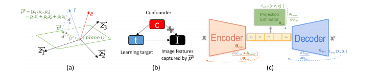
Fig. 1. The proposed AI approach for association analysis in medical imaging. (a) Geometry perspective of correlations between a target and a confounder variable (𝐭, 𝐜), andits extension (?𝑡, ?𝑐) into the latent space (n=3 latent dimensions) of an autoencoder. Plane O is orthogonal to ?𝑐. 𝑝?? is the vector projection of ?𝑡 onto plane O. 𝐝 is the latentrepresentation of an input image and 𝐝 ′ is its projection onto 𝑝?? . 𝑧 ? 𝑝 is the distance between 𝐝 ′ and the origin. For cases with 𝑚 confounders, the latent dimensions should be𝑛 ≥ 𝑚 + 1, so as to guarantee there exist a 𝑝?? orthogonal to 𝑚 confounders; (b) a directed acyclic diagram explains the relationships between 𝐭, 𝐜, and image I. We aim to extractimage features associated with the learning target while being independent to the confounders. (c) The proposed approach in a neural network perspective. [𝑧1 , 𝑧2 ,… , 𝑧𝑛 ] arethe learned latent features by the network, which construct the latent space shown in (a); 𝐗 and 𝐗′ refer to the input and reconstructed image; θ𝑒𝑛𝑐 , θ𝑑𝑒𝑐 , θ𝑝𝑒 are the trainableparameters of encoder, decoder, and projection estimator.

圖1. 所提出的用于醫學影像關聯分析的人工智能方法。(a) 目標變量和混雜變量（𝐭, 𝐜）之間相關性的幾何視角，以及它們在自動編碼器的潛在空間（潛在維度數(n = 3)）中的擴展（?𝑡, ?𝑐）。平面(O)與?𝑐正交。𝑝?? 是?𝑡在平面(O)上的向量投影。𝐝 是輸入圖像的潛在表征，𝐝 ′ 是它在𝑝?? 上的投影。𝑧 ? 𝑝 是 𝐝 ′ 與原點之間的距離。對于有(m)個混雜因素的情況，潛在維度數應滿足(n* \geq m + 1)，以確保存在一個與(m)個混雜因素正交的𝑝?? ；(b) 一個有向無環圖解釋了 𝐭, 𝐜 和圖像(I)之間的關系。我們的目標是提取與學習目標相關且獨立于混雜因素的圖像特征。(c) 從神經網絡的角度來看所提出的方法。[(𝑧1, 𝑧2, \ldots, 𝑧n)] 是網絡學習到的潛在特征，它們構成了圖 (a) 中所示的潛在空間；𝐗 和 𝐗′ 分別指輸入圖像和重建圖像；(\theta{enc})、(\theta{dec})、(\theta{pe}) 分別是編碼器、解碼器和投影估計器的可訓練參數。

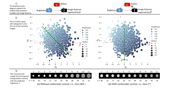
Fig. 2. The distribution of the 2-D latent space for the synthetic images in the test set of Experiment 1, and the eleven reconstructed images sampling along the brightness-relatedvector, (a) without (i.e., vector ?𝑝) and (b) with correction (vector 𝑝??) for the confounding of circle radius, together with the predicted brightness 𝑡? derived by Eq. (6) and Eq.(7). 𝑍1 -axis: the first dimension of the latent space; 𝑍2 -axis: the second dimension. Each data point in the latent space represents an input image, which is denoted by its radiusand brightness. After training, eleven frames were reconstructed by sampling eleven points along the vector ?𝑝 and 𝑝?? (Eq. (6) and Eq. (7)) to visualize the confounding effects.Whereas our method does not involve the estimation of vectors ?𝑡 and ?𝑐, we have manually included them in this figure only for the purpose of enhancing comprehension

圖2：實驗1測試集中合成圖像的二維潛在空間分布，以及沿亮度相關向量采樣得到的十一張重建圖像。(a) 未校正（即向量(\vec{p})）以及 (b) 校正后（向量(\vec{p}^)）對圓形半徑混雜因素的處理情況，同時展示了通過公式（6）和公式（7）得出的預測亮度(\hat{t})。(Z_1)軸：潛在空間的第一維度；(Z_2)軸：潛在空間的第二維度。潛在空間中的每個數據點代表一幅輸入圖像，由其半徑和亮度來表示。訓練完成后，沿著向量(\vec{p})和(\vec{p}^)（公式（6）和公式（7））采樣十一個點來重建十一幀圖像，以可視化混雜效應。盡管我們的方法不涉及向量(\vec{t})和(\vec{c})的估計，但我們在此圖中手動加入了它們，只是為了增強理解。

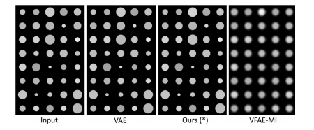
Fig. 3. The input images 𝐗 (8 × 5 circle images), and the reconstructed images 𝐗′ ofdifferent methods, in Experiment 1

圖3：實驗1中，輸入圖像 𝐗（8×5的圓形圖像）以及不同方法得到的重建圖像 𝐗′ 。

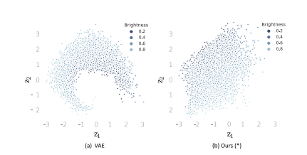
Fig. 4. Distribution of datapoints in the 2-D latent space via (a) unsupervised trainingand (b) our proposed supervised training, in Experiment 1.

圖4：實驗1中，通過(a)無監督訓練和(b)我們所提出的有監督訓練得到的二維潛在空間中數據點的分布情況。

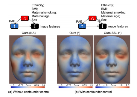
Fig. 5. Interpretation heatmaps of facial changes in children with PAE using theproposed method: (a) without correction for confounders; (b) with correction forethnicity, BMI, maternal smoking, maternal age, and sex. Red areas refer to inwardchanges of the face with respect to the geometric center of the head. Heatmapgeneration is detailed in Section

圖5：使用所提出的方法得到的孕期暴露于酒精（PAE）兒童面部變化的解釋熱圖：(a) 未校正混雜因素；(b) 校正了種族、身體質量指數（BMI）、母親吸煙情況、母親年齡和性別的混雜因素。紅色區域表示面部相對于頭部幾何中心的向內變化情況。熱圖的生成細節見[具體章節] 。

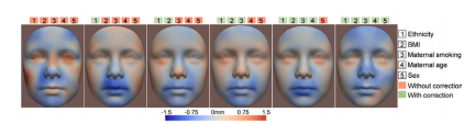
Fig. 6. Interpretation heatmaps of facial changes in children exposed to alcohol duringpregnancy (PAE) using the proposed method with gradual correction for confoundersof ethnicity, BMI, maternal smoking, maternal age, and sex. From left to right, in thefirst heatmap no confounder was corrected for during the training; in the last heatmapall five confounders were corrected Eq. (4). Red areas refer to inward changes of theface with respect to the geometric center of the head

圖6：使用我們所提出的方法，針對孕期暴露于酒精（PAE）的兒童面部變化的解釋熱圖，該方法逐步校正了種族、身體質量指數（BMI）、母親吸煙情況、母親年齡和性別的混雜因素。從左至右，在第一張熱圖中，訓練期間未校正任何混雜因素；在最后一張熱圖中，對公式（4）中的所有五個混雜因素都進行了校正。紅色區域表示面部相對于頭部幾何中心的向內變化情況。

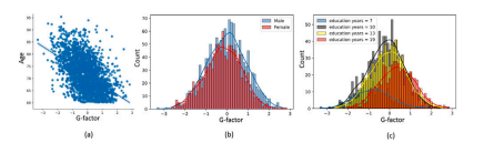
Fig. 7. Data characteristic of the study population. (a) Joint distribution of g-factor andage. The Pearson’s correlation coefficient between age and g-factor is ?0.51 (p-value= 4.88e?163, linear regression); (b) Histogram distribution of g-factor between maleand female. Male show slightly higher g-factor than female (p-value = 1.4e?5, linearregression); (c) Histogram distribution of g-factor for different educational years. Highereducational years show overall higher g-factors (p-value = 2.87e?57, linear regression)

圖7：研究人群的數據特征。(a) 一般智力因素（g因素）與年齡的聯合分布。年齡與g因素之間的皮爾遜相關系數為?0.51（(p)值 = (4.88×10^{-163})，線性回歸）；(b) 男性和女性之間g因素的直方圖分布。男性的g因素略高于女性（(p)值 = (1.4×10^{-5})，線性回歸）；(c) 不同受教育年限人群的g因素直方圖分布。受教育年限越高，總體上g因素也越高（(p)值 = (2.87×10^{-57})，線性回歸）。

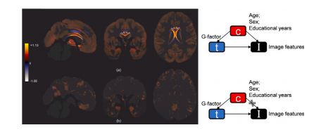
Fig. 8.Reconstructed supratentorial modulated gray matter maps using the sampledlatent features along the direction of increasing g-factor (a) without correcting forconfounders, and (b) with correcting for age, sex, and educational years. The resultsare averaged over the five folds, and masked out the statistically non-significant region.Color bar shows the direction and magnitude of the changes of GM density associatedwith a higher g-factor.

圖8：利用沿g因素增加方向采樣的潛在特征重建的幕上調制灰質圖。(a) 未校正混雜因素，(b) 校正了年齡、性別和受教育年限。結果是五折交叉驗證的平均值，并屏蔽了統計上不顯著的區域。色條顯示了與較高g因素相關的灰質密度變化的方向和幅度。?

Table

表

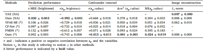
Table 1Prediction error, Pearson’s correlation coefficient, and image reconstruction quality of methods without (NA) and with (*) correction for thecircle radius (confounder) in predicting the circle brightness (learning target) on the test set

表1：在測試集上，針對預測圓形亮度（學習目標）時，未校正（NA）和已校正（*）圓形半徑（混雜因素）的各方法的預測誤差、皮爾遜相關系數以及圖像重建質量

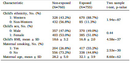
Table 2Data characteristic of children and their mothers included in the analysis (for thelabeled data only, N=1,515).

表2：納入分析的兒童及其母親的數據特征（僅針對標記數據，(N = 1515)） 。

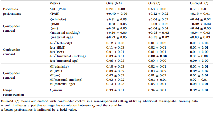
Table 3Association analysis between PAE (learning target) and children’s facial shape (input image). Results are presented without (NA) and with (*)controlling of the confounders (ethnicity, BMI, sex, maternal smoking, maternal age).

表3：孕期酒精暴露（PAE，學習目標）與兒童面部形狀（輸入圖像）之間的關聯分析。結果展示了未（NA）和已（*）控制混雜因素（種族、身體質量指數、性別、母親吸煙情況、母親年齡）的情況。

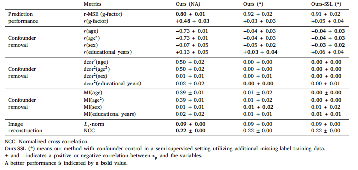
Table 4Association analysis between the learning target global cognition (g-factor) and brain gray matter imaging. Results are presented without (NA)and with (*) controlling of confounders (age, sex, and educational years)

表4：學習目標即整體認知能力（g因素）與腦灰質成像之間的關聯分析。結果呈現了未（NA）和已（*）控制混雜因素（年齡、性別和受教育年限）的情況。