目錄
- Probability and Bayes’ Rule
- Introduction
- Probabilities
- Probability of the intersection
- Bayes’ Rule
- Conditional Probabilities
- Bayes’ Rule
- Quiz: Bayes’ Rule Applied
- Na?ve Bayes Introduction
- Na?ve Bayes for Sentiment Analysis
- P ( w i ∣ c l a s s ) P(w_i|class) P(wi?∣class)
- Na?ve Bayes
- Laplacian Smoothing
- Laplacian Smoothing
- Introducing P ( w i ∣ c l a s s ) P(w_i|class) P(wi?∣class) with smoothing
- Log Likelihood
- Ratio of probabilities
- Na?ve Bayes’ inference
- Log Likelihood, Part1
- Calculating Lambda
- Summary
- Log Likelihood, Part 2
- Training Na?ve Bayes
- Testing Na?ve Bayes
- Predict using Na?ve Bayes
- Testing Na?ve Bayes
- Applications of Na?ve Bayes
- Na?ve Bayes Assumptions
- Error Analysis
- Punctuation
- Removing Words
- Adversarial attacks
Probability and Bayes’ Rule
概率與條件概率及其數學表達
貝葉斯規則(應用于不同領域,包括 NLP)
建立自己的 Naive-Bayes 推文分類器
Introduction
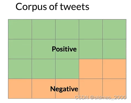
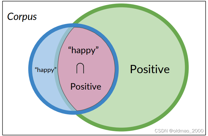
假設我們有一個推文語料庫,里面包含正面和負面情感的推文:
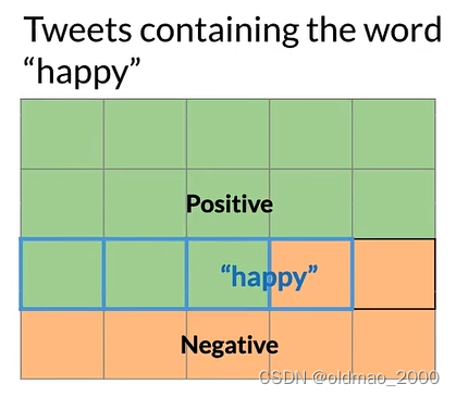
某個單詞例如:happy,可能出現在正面或負面情感的推文中:
下面我們用數學公式來表示上面的概率描述。
Probabilities
A A A表示正面的推文,則正面的推文發生的概率可以表示為:
P ( A ) = P ( P o s i t i v e ) = N p o s / N P(A)=P(Positive)=N_{pos}/N P(A)=P(Positive)=Npos?/N
以上圖為例:
P ( A ) = N p o s / N = 13 / 20 = 0.65 P(A)=N_{pos}/N=13/20=0.65 P(A)=Npos?/N=13/20=0.65
而負面推文發生的概率可以表示為:
P ( N e g a t i v e ) = 1 ? P ( P o s i t i v e ) = 0..35 P(Negative)=1-P(Positive)=0..35 P(Negative)=1?P(Positive)=0..35
happy可能出現在正面或負面情感的推文中可以表示為 B B B:
則 B B B發生概率可以表示為:
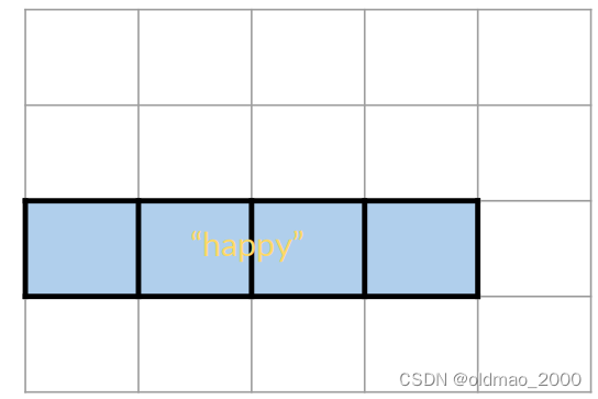
P ( B ) = P ( h a p p y ) = N h a p p y / N P ( B ) = 4 / 20 = 0.2 P(B) = P(happy) = N_{happy}/N\\ P(B) =4/20=0.2 P(B)=P(happy)=Nhappy?/NP(B)=4/20=0.2
Probability of the intersection
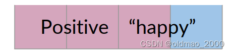
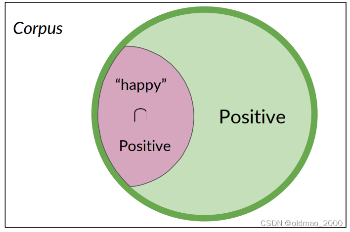
下面表示正面推文且包含單詞happy可圖形化表示為:
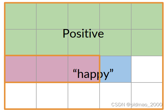
也可以用交集的形式表示:
P ( A ∩ B ) = P ( A , B ) = 3 20 = 0.15 P(A\cap B)=P(A,B)=\cfrac{3}{20}=0.15 P(A∩B)=P(A,B)=203?=0.15
語料庫中有20條推文,其中有3條被標記為積極且同時包含單詞happy
Bayes’ Rule
Conditional Probabilities
如果我們在三亞,并且現在是冬天,你可以猜測天氣如何,那么你的猜測比只直接猜測天氣要準確得多。
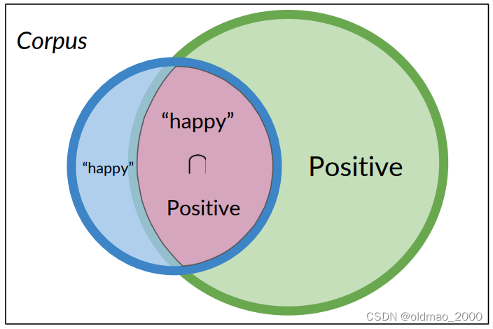
用推文的例子來說:
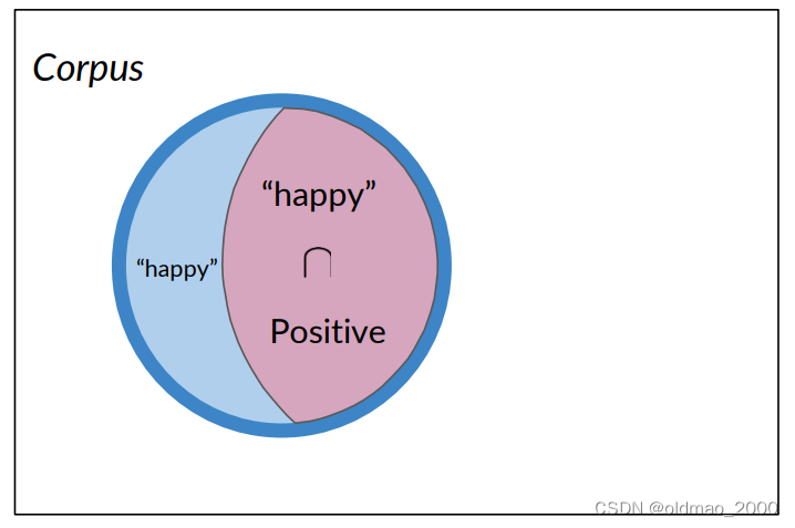
如果只考慮包含單詞happy的推文(4條),而不是整個語料庫,考慮這個里面包含正面推文的概率:
P ( A ∣ B ) = P ( P o s i t i v e ∣ “ h a p p y " ) P ( A ∣ B ) = 3 / 4 = 0.75 P(A|B)=P(Positive|“happy")\\ P(A|B)=3/4=0.75 P(A∣B)=P(Positive∣“happy")P(A∣B)=3/4=0.75
反過來說,只考慮正面推文,看其出現happy單詞的推文概率:
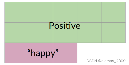
P ( B ∣ A ) = P ( “ h a p p y ” ∣ P o s i t i v e ) P ( B ∣ A ) = 3 / 13 = 0.231 P(B | A) = P(“happy”| Positive) \\ P(B | A) = 3 / 13 = 0.231 P(B∣A)=P(“happy”∣Positive)P(B∣A)=3/13=0.231
從上面例子可以看到:條件概率可以被解釋為已知事件A已經發生的情況下,結果B發生的概率,或者從集合A中查看一個元素,它同時屬于集合B的概率。
Probability of B, given A happened
Looking at the elements of set A, the chance that one also belongs to set B
P ( P o s i t i v e ∣ “ h a p p y " ) = P ( P o s i t i v e ∩ “ h a p p y " ) P ( “ h a p p y " ) P(Positive|“happy")=\cfrac{P(Positive\cap “happy")}{P(“happy")} P(Positive∣“happy")=P(“happy")P(Positive∩“happy")?
Bayes’ Rule
使用條件概率推導貝葉斯定理
同理:
P ( P o s i t i v e ∣ “ h a p p y " ) = P ( P o s i t i v e ∩ “ h a p p y " ) P ( “ h a p p y " ) P(Positive|“happy")=\cfrac{P(Positive\cap “happy")}{P(“happy")} P(Positive∣“happy")=P(“happy")P(Positive∩“happy")?
P ( “ h a p p y " ∣ P o s i t i v e ) = P ( “ h a p p y " ∩ P o s i t i v e ) P ( P o s i t i v e ) P(“happy"|Positive)=\cfrac{P( “happy"\cap Positive)}{P(Positive)} P(“happy"∣Positive)=P(Positive)P(“happy"∩Positive)?
上面兩個式子的分子表示的數量是一樣的。
有了以上公式則可以推導貝葉斯定理。
P ( P o s i t i v e ∣ “ h a p p y " ) = P ( “ h a p p y " ∣ P o s i t i v e ) × P ( P o s i t i v e ) P ( “ h a p p y " ) P(Positive|“happy")=P(“happy"|Positive)\times\cfrac{P(Positive)}{P(“happy")} P(Positive∣“happy")=P(“happy"∣Positive)×P(“happy")P(Positive)?
通用形式為:
P ( X ∣ Y ) = P ( Y ∣ X ) × P ( X ) P ( Y ) P(X|Y)=P(Y|X)\times \cfrac{P(X)}{P(Y)} P(X∣Y)=P(Y∣X)×P(Y)P(X)?
Quiz: Bayes’ Rule Applied
Suppose that in your dataset, 25% of the positive tweets contain the word ‘happy’. You also know that a total of 13% of the tweets in your dataset contain the word ‘happy’, and that 40% of the total number of tweets are positive. You observe the tweet: '‘happy to learn NLP’. What is the probability that this tweet is positive?
A: P(Positive | “happy” ) = 0.77
B: P(Positive | “happy” ) = 0.08
C: P(Positive | “happy” ) = 0.10
D: P(Positive | “happy” ) = 1.92
答案:A
Na?ve Bayes Introduction
學會使用Na?ve Bayes來進行二分類(使用概率表)
Na?ve Bayes for Sentiment Analysis
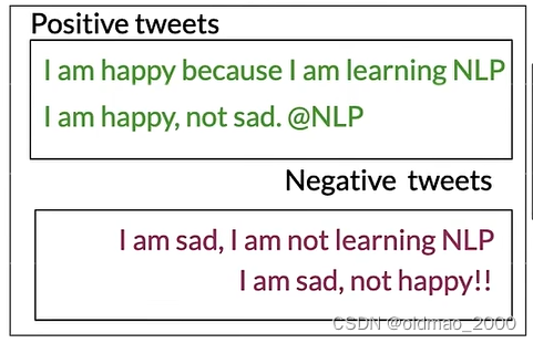
假設有以下語料:
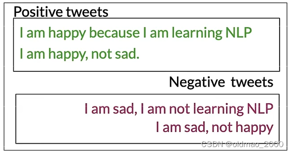
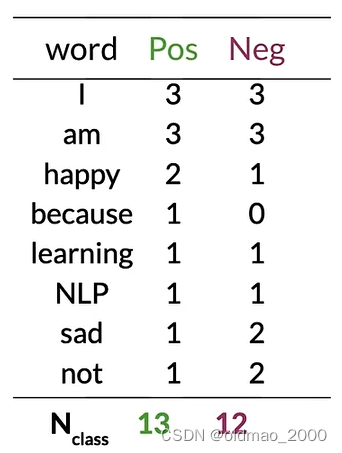
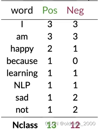
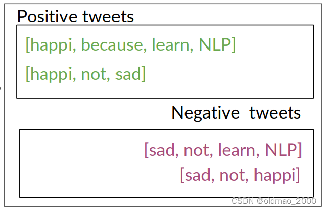
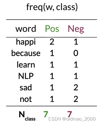
按C1W1中提到方法提取詞庫,并統計正負面詞頻:
P ( w i ∣ c l a s s ) P(w_i|class) P(wi?∣class)
將類別中每個單詞的頻率除以它對應的類別中單詞的總數。
例如:對于單詞"I",正面類別的條件概率將是3/13:
p ( I ∣ P o s ) = 3 13 = 0.24 p(I|Pos)=\cfrac{3}{13}=0.24 p(I∣Pos)=133?=0.24
對于負面類別中的單詞"I",可以得到3/12:
p ( I ∣ N e g ) = 3 12 = 0.25 p(I|Neg)=\cfrac{3}{12}=0.25 p(I∣Neg)=123?=0.25
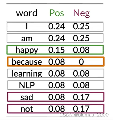
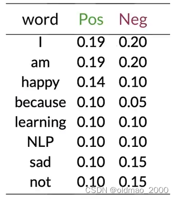
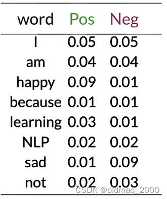
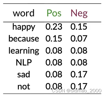
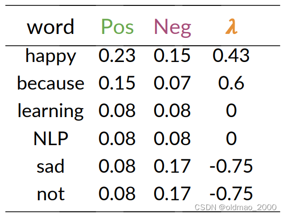
將以上內容保存為表(because的Neg概率不太對,應該是0):
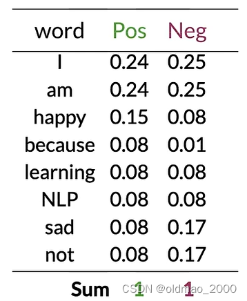
可以看到有很多單詞(中性詞)在表中的Pos和Neg的值大約相等(Pos≈Neg),例如:I、am、learning、NLP。
這些具有相等概率的單詞對情感沒有任何貢獻。
而單詞happy、sad、not的Pos和Neg的值差異很大,這些詞對于確定推文的情感具有很大影響,綠色是積極影響,紫色是負面影響。
對于單詞because,其 p ( I ∣ N e g ) = 0 12 = 0 p(I|Neg)=\cfrac{0}{12}=0 p(I∣Neg)=120?=0
這情況在計算貝葉斯概率的時候會出現分母為0的情況,為避免這個情況發生,可以引入平滑處理。
Na?ve Bayes
假如有以下推文:
I am happy today; I am learning.
按上面的計算方式得到詞表以及其Pos和Neg的概率值:
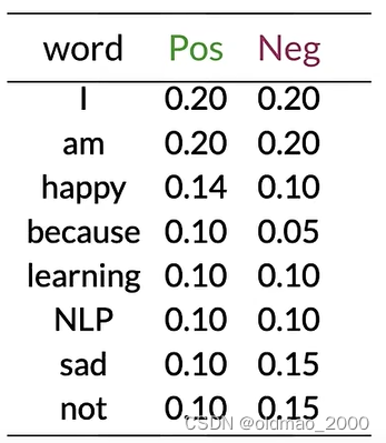
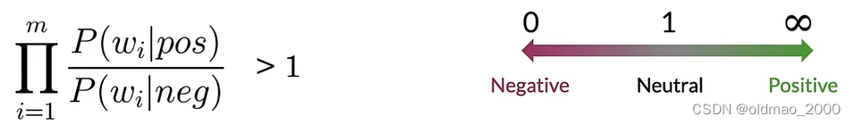
使用以下公式計算示例推文的情感:
∏ i = 1 m P ( w i ∣ p o s ) P ( w i ∣ n e g ) \prod_{i=1}^m\cfrac{P(w_i|pos)}{P(w_i|neg)} i=1∏m?P(wi?∣neg)P(wi?∣pos)?
就是計算推文每個單詞的第二列比上第三列,然后連乘。
示例推文today不在詞表中,忽略,其他單詞帶入公式:
0.20 0.20 × 0.20 0.20 × 0.14 0.10 × 0.20 0.20 × 0.20 0.20 × 0.10 0.10 = 0.14 0.10 = 1.4 > 1 \cfrac{0.20}{0.20}\times\cfrac{0.20}{0.20}\times\cfrac{0.14}{0.10}\times\cfrac{0.20}{0.20}\times\cfrac{0.20}{0.20}\times\cfrac{0.10}{0.10}=\cfrac{0.14}{0.10}=1.4>1 0.200.20?×0.200.20?×0.100.14?×0.200.20?×0.200.20?×0.100.10?=0.100.14?=1.4>1
可以看到,中性詞對預測結果沒有任何作用,最后結果大于1,表示示例推文是正面的。
Laplacian Smoothing
Laplacian Smoothing主要用于以下目的:
避免零概率問題:在統計語言模型中,某些詞或詞序列可能從未在訓練數據中出現過,導致其概率為零。拉普拉斯平滑通過為所有可能的事件分配一個非零概率來解決這個問題。
概率分布估計:拉普拉斯平滑提供了一種簡單有效的方法來估計概率分布,即使在數據不完整或有限的情況下。
平滑處理:它通過為所有可能的事件添加一個小的常數(通常是1),來平滑概率分布,從而減少極端概率值的影響。
提高模型的泛化能力:通過避免概率為零的情況,拉普拉斯平滑有助于提高模型對未見數據的泛化能力。
簡化計算:拉普拉斯平滑提供了一種簡單的方式來調整概率,使得計算和實現相對容易。
Laplacian Smoothing
計算給定類別下一個詞的條件概率的表達式是詞在語料庫中出現的頻率:
P ( w i ∣ c l a s s ) = f r e q ( w i , c l a s s ) N c l a s s c l a s s ∈ { P o s i t i v e , N e g a t i v e } P(w_i|class)=\cfrac{freq(w_i,class)}{N_{class}}\quad class\in\{Positive,Negative\} P(wi?∣class)=Nclass?freq(wi?,class)?class∈{Positive,Negative}
其中 N c l a s s N_{class} Nclass?是frequency of all words in class
加入平滑項后公式寫為:
P ( w i ∣ c l a s s ) = f r e q ( w i , c l a s s ) + 1 N c l a s s + V c l a s s P(w_i|class)=\cfrac{freq(w_i,class)+1}{N_{class}+V_{class}} P(wi?∣class)=Nclass?+Vclass?freq(wi?,class)+1?
V c l a s s V_{class} Vclass?是number of unique words in class
分子項+1避免了概率為0的情況,但是會導致總概率不等于1的情況,為了避免這個情況,在分母中加了 V c l a s s V_{class} Vclass?
Introducing P ( w i ∣ c l a s s ) P(w_i|class) P(wi?∣class) with smoothing
使用之前的例子。
上表中共有8個不同單詞, V = 8 V=8 V=8
對于單詞I則有:
P ( I ∣ P o s ) = 3 + 1 13 + 8 = 0.19 P ( I ∣ N e g ) = 3 + 1 12 + 8 = 0.20 P(I|Pos)=\cfrac{3+1}{13+8}=0.19\\ P(I|Neg)=\cfrac{3+1}{12+8}=0.20 P(I∣Pos)=13+83+1?=0.19P(I∣Neg)=12+83+1?=0.20
同理可以計算出其他單詞平滑厚度結果:
雖然結果已經四舍五入,但是兩列概率值總和還是為1
Log Likelihood
Ratio of probabilities
根據之前講的內容,我們知道每個單詞可以按其Pos和Neg的值的差異分為三類,正面、負面和中性詞。
我們把這個差異用下面公式表示:
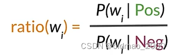
然后,我們可以計算上面概率表中的ratio(吐槽一下,這里because的概率不知道怎么搞的老是變來變去)
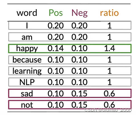
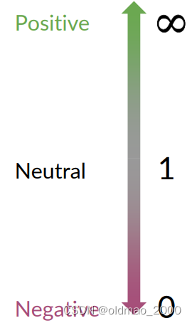
ratio取值與分類的關系很簡單:
Na?ve Bayes’ inference
下面給出完整的樸素貝葉斯二元分類公式:
P ( p o s ) P ( n e g ) ∏ i = 1 m P ( w i ∣ p o s ) P ( w i ∣ n e g ) > 1 c l a s s ∈ { p o s , n e g } w → Set?of?m?words?in?a?tweet \cfrac{P(pos)}{P(neg)}\prod_{i=1}^m\cfrac{P(w_i|pos)}{P(w_i|neg)}>1\quad class\in\{pos,neg\}\quad w\rightarrow\text{Set of m words in a tweet} P(neg)P(pos)?i=1∏m?P(wi?∣neg)P(wi?∣pos)?>1class∈{pos,neg}w→Set?of?m?words?in?a?tweet
左邊一項其實是先驗概率,如果數據集中正負樣本差不多,則該項比值為1,可以忽略。這個比率可以看作是模型在沒有任何其他信息的情況下,傾向于認為推文是正面或負面情感的初始信念。;
右邊一項之前已經推導過。這是條件概率的乘積。對于推文中的每個詞 w i , i = 1 , 2 , ? , m w_i,i=1,2,\cdots,m wi?,i=1,2,?,m(m 是推文中的詞的數量),這個乘積計算了在正面情感條件下該詞出現的概率與在負面情感條件下該詞出現的概率的比值。這個乘積考慮了推文中所有詞的證據
如果這個乘積大于1,那么模型認為推文更可能是正面情感;如果小于1,則更可能是負面情感。
Log Likelihood, Part1
上面的樸素貝葉斯二元分類公式使用了連乘的形式,對于計算上說,小數的連乘會使得計算出現underflow,根據對數性質:
log ? ( a ? b ) = log ? ( a ) + log ? ( b ) \log(a*b)=\log(a)+\log(b) log(a?b)=log(a)+log(b)
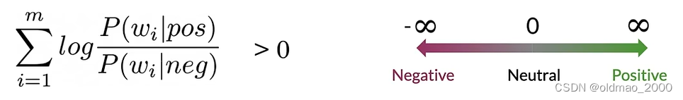
可以將連乘轉化成為連加的形式,同樣對公式求對數得到:
log ? ( P ( p o s ) P ( n e g ) ∏ i = 1 m P ( w i ∣ p o s ) P ( w i ∣ n e g ) ) = log ? P ( p o s ) P ( n e g ) + ∑ i = 1 m log ? P ( w i ∣ p o s ) P ( w i ∣ n e g ) \log\left(\cfrac{P(pos)}{P(neg)}\prod_{i=1}^m\cfrac{P(w_i|pos)}{P(w_i|neg)}\right)=\log\cfrac{P(pos)}{P(neg)}+\sum_{i=1}^m\log\cfrac{P(w_i|pos)}{P(w_i|neg)} log(P(neg)P(pos)?i=1∏m?P(wi?∣neg)P(wi?∣pos)?)=logP(neg)P(pos)?+i=1∑m?logP(wi?∣neg)P(wi?∣pos)?
也就是:log prior + log likelihood
我們將第一項成為: λ \lambda λ
Calculating Lambda
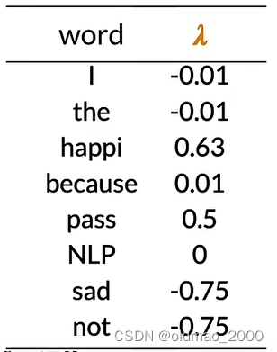
根據上面的內容計算實例推文的lambda:
tweet: I am happy because I am learning.
先計算出概率表:
然后根據公式計算出每個單詞的 λ \lambda λ:
λ ( w ) = log ? P ( w ∣ p o s ) P ( w ∣ n e g ) \lambda(w)=\log\cfrac{P(w|pos)}{P(w|neg)} λ(w)=logP(w∣neg)P(w∣pos)?
例如對于第一個單詞:
λ ( I ) = log ? 0.05 0.05 = log ? ( 1 ) = 0 \lambda(I)=\log\cfrac{0.05}{0.05}=\log(1)=0 λ(I)=log0.050.05?=log(1)=0
happy:
λ ( h a p p y ) = log ? 0.09 0.01 = log ? ( 9 ) = 2.2 \lambda(happy)=\log\cfrac{0.09}{0.01}=\log(9)=2.2 λ(happy)=log0.010.09?=log(9)=2.2
以此類推:
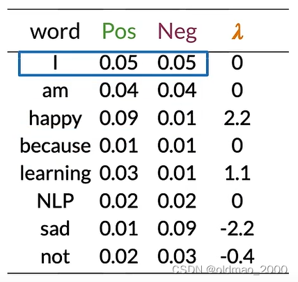
可以看到,這里我們也可以根據 λ \lambda λ值來判斷正負面和中性詞。
Summary
對于正負面、中性詞,這里給出兩種判斷方式(Word sentiment):
r a t i o ( w ) = P ( w ∣ p o s ) P ( w ∣ n e g ) ratio(w)=\cfrac{P(w|pos)}{P(w|neg)} ratio(w)=P(w∣neg)P(w∣pos)?
λ ( w ) = log ? P ( w ∣ p o s ) P ( w ∣ n e g ) \lambda(w)=\log\cfrac{P(w|pos)}{P(w|neg)} λ(w)=logP(w∣neg)P(w∣pos)?
這里要明白,為什么要使用第二種判斷方式:避免underflow(下溢)
Log Likelihood, Part 2
有了 λ \lambda λ值,接下來可以計算對數似然,對于以下推文:
I am happy because I am learning.
其每個單詞 λ \lambda λ值在上面的圖中,整個推文的對數似然值就是做累加:
0 + 0 + 2.2 + 0 + 0 + 0 + 1.1 = 3.3 0+0+2.2+0+0+0+1.1=3.3 0+0+2.2+0+0+0+1.1=3.3
從前面我們可以知道,概率比值以及對數似然的值如何區分正負樣本:
這里的推文對數似然的值為3.3,是一個正面樣本。
Training Na?ve Bayes
這里不用GD,只需簡單五步完成訓練模型。
Step 0: Collect and annotate corpus
Step 1: Preprocess
包括:
Lowercase
Remove punctuation, urls, names
Remove stop words
Stemming
Tokenize sentences
Step 2: Word count
Step 3: P ( w ∣ c l a s s ) P(w|class) P(w∣class)
這里 V c l a s s = 6 V_{class}=6 Vclass?=6
根據公式:
f r e q ( w , c l a s s ) + 1 N c l a s s + V c l a s s \cfrac{freq(w,class)+1}{N_{class}+V_{class}} Nclass?+Vclass?freq(w,class)+1?
計算概率表:
Step 4: Get lambda
根據公式:
λ ( w ) = log ? P ( w ∣ p o s ) P ( w ∣ n e g ) \lambda(w)=\log\cfrac{P(w|pos)}{P(w|neg)} λ(w)=logP(w∣neg)P(w∣pos)?
得到:
Step 5: Get the log prior
估計先驗概率,分別計算:
D p o s D_{pos} Dpos? = Number of positive tweets
D n e g D_{neg} Dneg? = Number of negative tweets
log?prior = log ? D p o s D n e g \text{log prior}=\log\cfrac{D_{pos}}{D_{neg}} log?prior=logDneg?Dpos??
注意:
If dataset is balanced, D p o s = D n e g D_{pos}=D_{neg} Dpos?=Dneg? and log?prior = 0 \text{log prior}=0 log?prior=0.
對應正負樣本不均衡的數據庫,先驗概率不能忽略
總的來看是六步:
- Get or annotate a dataset with positive and negative tweets
- Preprocess the tweets: p r o c e s s _ t w e e t ( t w e e t ) ? [ w 1 , w 2 , w 3 , . . . ] process\_tweet(tweet) ? [w_1 , w_2 , w_3 , ...] process_tweet(tweet)?[w1?,w2?,w3?,...]
- Compute freq(w, class),注意要引入拉普拉斯平滑
- Get P(w | pos), P(w | neg)
- Get λ(w)
- Compute log prior = log(P(pos) / P(neg))
Testing Na?ve Bayes
Predict using Na?ve Bayes
進行之前的步驟,我們完成了詞典中每個單詞對數似然λ(w)的計算,并形成了字典。
假設我們數據集中正負樣本基本均衡,可以忽略對數先驗概率( log?prior = 0 \text{log prior}=0 log?prior=0)
對于推文:
[I, pass, the , NLP, interview]
計算其對數似然為:
s c o r e = ? 0.01 + 0.5 ? 0.01 + 0 + log?prior = 0.48 score = -0.01+0.5-0.01+0+\text{log prior}=0.48 score=?0.01+0.5?0.01+0+log?prior=0.48
其中interview為未知詞,忽略。
也就是是預測值為0.48>0,該推文是正面的。
Testing Na?ve Bayes
假設有驗證集數據: X v a l X_{val} Xval?和標簽 Y v a l Y_{val} Yval?
計算 λ \lambda λ和log prior,對于未知詞要忽略(也就相當于看做是中性詞)
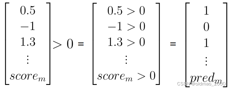
計算 s c o r e = p r e d i c t ( X v a l , λ , log?prior ) score=predict(X_{val},\lambda,\text{log prior}) score=predict(Xval?,λ,log?prior)
判斷推文情感: p r e d = s c o r e > 0 pred = score>0 pred=score>0
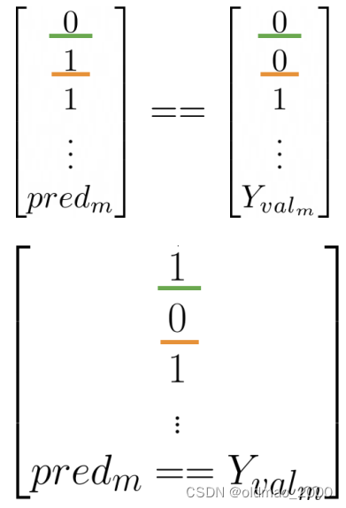
計算模型正確率:
1 m ∑ i = 1 m ( p r e d i = = Y v a l i ) \cfrac{1}{m}\sum_{i=1}^m(pred_i==Y_{val_i}) m1?i=1∑m?(predi?==Yvali??)
Applications of Na?ve Bayes
除了Sentiment analysis
Na?ve Bayes常見應用還包括:
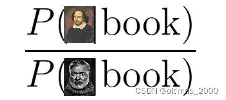
● Author identification
如果有兩個大型文集,分別由不同的作者撰寫,可以訓練一個模型來識別新文檔是由哪一位寫的。
例如:你手頭上有一些莎士比亞的作品和海明威的作品,你可以計算每個詞的Lambda值,以預測個新詞被莎士比亞使用的可能性,或者被海明威使用的可能性。
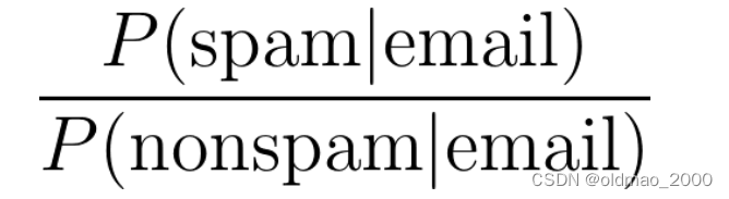
●Spam filtering:
● Information retrieval
樸素貝葉斯最早的應用之一是在數據庫中根據查詢中的關鍵字將文檔篩選為相關和不相關的文檔。
這里只需要計算文檔的對數似然,因為先驗是未知的。
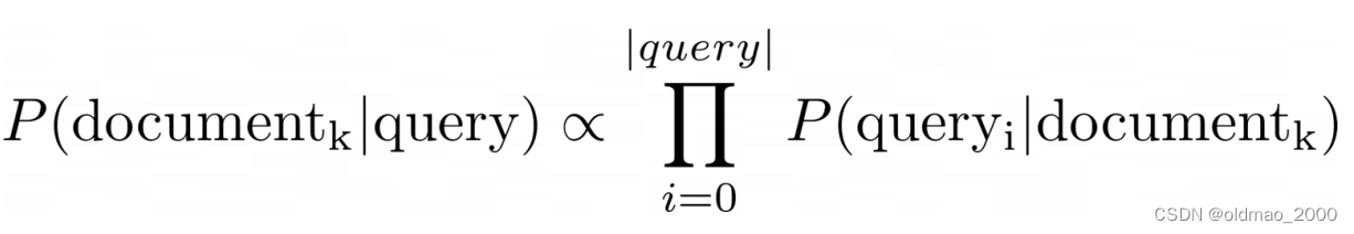
然后根據閾值判斷是否查詢文檔:

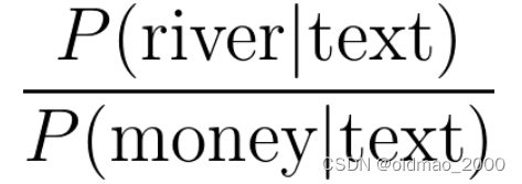
● Word disambiguation
假設單詞在文中有兩種含義,詞義消岐可以判斷單詞在上下文的含義。

bank有河岸和銀行兩種意思。
Na?ve Bayes Assumptions
樸素貝葉斯是一個非常簡單的模型,它不需要設置任何自定義參數,因為它對數據做了一些假設。
● Independence
● Relative frequency in corpus
對于獨立性,樸素貝葉斯假設文本中的詞語是彼此獨立的。看下面例子:
“It is sunny and hot in the Sahara desert.”
單詞sunny 和hot 是有關聯性的,兩個詞語在一起可能與其所描述的事物有關,例如:海灘、甜點等。
樸素貝葉斯獨立性的假設可能會導致對個別詞語的條件概率估計不準確。

例如上圖中,winter的概率明顯要高于其他單詞,但樸素貝葉斯則認為四個單詞概率一樣。
另外一個問題是依賴于訓練數據集的分布。
理想的數據集中應該包含與隨機樣本相同比例的積極和消極推文,但是實際的推文中,正面推文要比負面推文出現頻率要更高。這樣訓練出來的模型會被戴上有色眼鏡。
Error Analysis
造成預測失敗的原因有三種:
● Removing punctuation and stop words
● Word order
● Adversarial attacks
Punctuation
Tweet: My beloved grandmother : (
經過標點處理后:processed_tweet: [belov, grandmoth]
我親愛的祖母,本來是正面推文,但是后面代表悲傷的emoj被過濾掉了。如果換成感嘆號那就不一樣。
Removing Words
Tweet: This is not good, because your attitude is not even close to being nice.
去掉停用詞后:processed_tweet: [good, attitude, close, nice]
Tweet: I am happy because I do not go.
Tweet: I am not happy because I did go.
上面一個是正面的(I am happy),后面一個是負面的(I am not happy)
否定詞和詞序會導致預測錯誤。
Adversarial attacks
主要是Sarcasm, Irony and Euphemisms(諷刺、反諷和委婉語),天才Sheldon都不能李姐!!!
Tweet: This is a ridiculously powerful movie. The plot was gripping and I cried right through until the ending!
processed_tweet: [ridicul, power, movi, plot, grip, cry, end]
原文表達是正面的: 這是一部震撼人心的電影。情節扣人心弦,我一直哭到結局!
但處理后的單詞卻是負面的。


,電生明火,無需燃料)
;里面10代表的涵義,以及其他可以賦值數字可以是多少?)