1 開發背景
VGGNet是牛津大學視覺幾何組(Visual Geometry Group)提出的模型,該模型在2014ImageNet圖像分類與定位挑戰賽 ILSVRC-2014中取得在分類任務第二,定位任務第一的優異成績。其核心貢獻在于系統性地探索了網絡深度對性能的影響,并證明了通過堆疊非常小的卷積核(3x3)可以顯著提升網絡性能。
論文地址:1409.1556] Very Deep Convolutional Networks for Large-Scale Image Recognition![]() https://arxiv.org/abs/1409.1556
https://arxiv.org/abs/1409.1556
論文詳解:(51 封私信 / 60 條消息) 經典神經網絡超詳細解讀(五)VGG網絡(論文精讀+網絡詳解+代碼實戰) - 知乎![]() https://zhuanlan.zhihu.com/p/27715976701
https://zhuanlan.zhihu.com/p/27715976701
2 網絡結構
2.1 VGG的核心思想
-
采用更深的網絡結構:相比 AlexNet(8 層),VGG 增加到了 16 或 19 層,提升了網絡的表達能力。
-
使用小卷積核(3×3)和多個連續的卷積層:所有卷積層都使用 3×3 卷積核,而不是較大的 5×5 或 7×7,這樣可以:
-
每個卷積層后面通常跟著一個ReLU激活函數,多個卷積層可以增加非線性能力(兩個 3×3 卷積相當于一個 5×5 卷積);
-
與使用大尺寸卷積核的單一層相比,多個小卷積層的堆疊可以提供更好的特征提取能力;
-
減少參數數量(比單個 5×5 卷積的參數更少)。
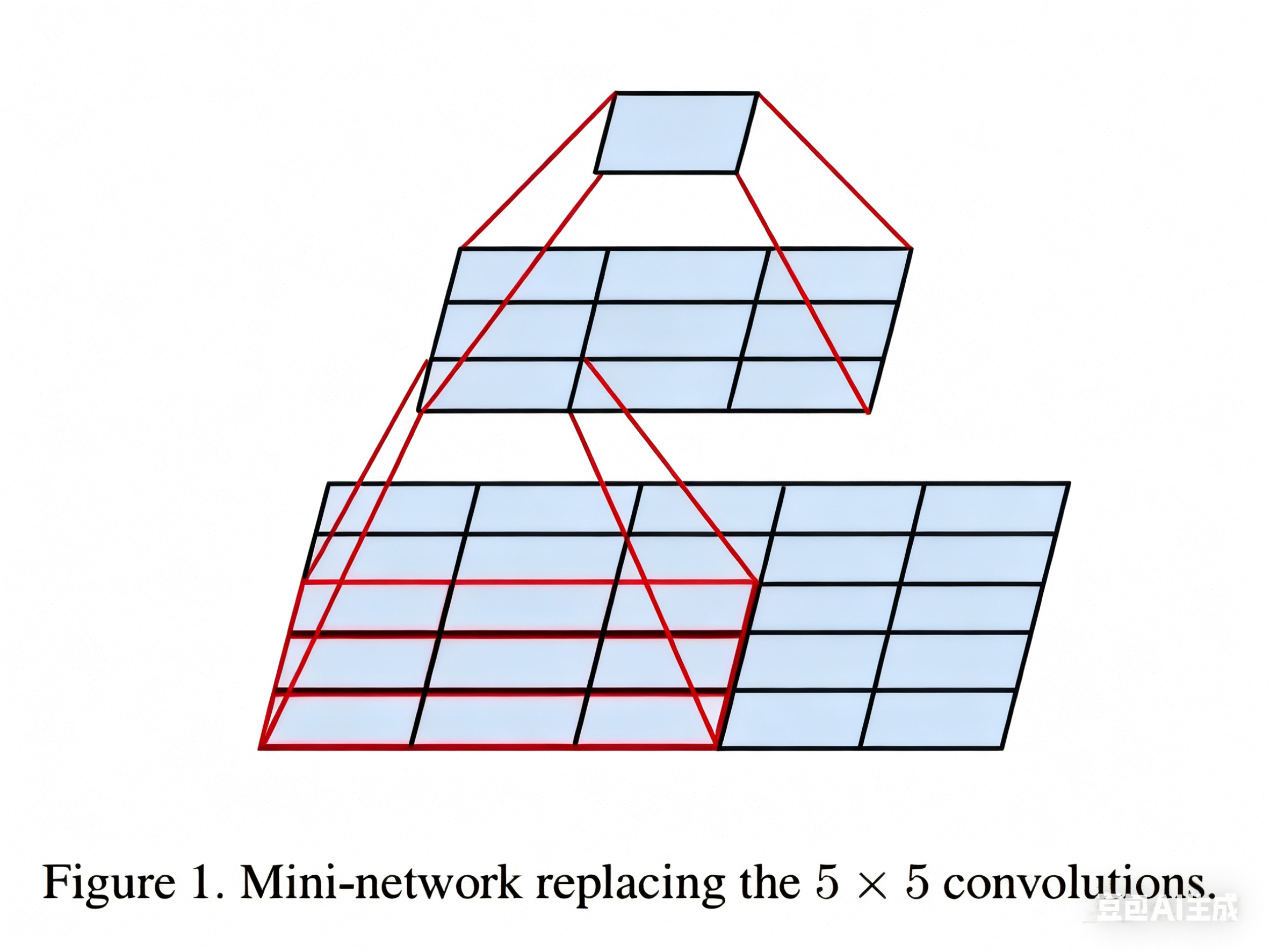
這里說明一下為什么兩個 3×3 卷積相當于一個 5×5 卷積,以及為什么參數數量變少了:
如上圖所示,如果我們使用一個 5×5 的卷積核對一個 5×5 的圖像進行卷積,最后可以得到一個 1×1 的輸出,而使用 3×3 的卷積核進行兩次連續的卷積,同樣可以得到 1×1 的輸出。同理,三個 3×3 的卷積相當于一個 7×7 的卷積。一個3×3卷積核在處理具有64個輸入通道的特征圖時,只有577(3×3×64+1=577,加的1是偏置項)個參數,而一個11x11的卷積核則有7745(11×11×64+1)個參數,7745>577×2。這種參數數量的顯著差異意味著使用小卷積核可以大幅減少網絡的參數量。
2.2 VGG架構實驗
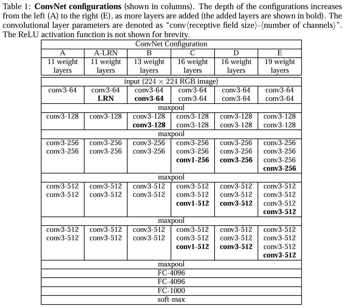
上圖是論文中六次實驗的結果圖。VGG網絡的卷積層全部為3*3的卷積核,用conv3-xxx來表示,xxx表示通道數。
-
第一組(A)就是個簡單的卷積神經網絡,沒有啥花里胡哨的地方。
-
第二組(A-LRN)在第一組的卷積神經網絡的基礎上加了LRN(LRN:局部響應歸一化,一種正則化手段,現在已不是主流了,LRN是Alexnet中提出的方法,在Alexnet中有不錯的表現 )
-
第三組(B)在A的基礎上加了兩個conv3,即多加了兩個3*3卷積核
-
第四組(C)在B的基礎上加了三個conv1,即多加了三個1*1卷積核
-
第五組(D)在C的基礎上把三個conv1換成了三個3*3卷積核
-
第六組(E)在D的基礎上又加了三個conv3,即多加了三個3*3卷積核
結論:
1.第一組和第二組進行對比,LRN在這里并沒有很好的表現;
2.第四組和第五組進行對比,conv3比conv1好使;
3.統籌看這六組實驗,會發現隨著網絡層數的加深,模型的表現會越來越好。
據此可簡單總結:作者一共實驗了6種網絡結構,其中VGG16(D)和VGG19(E)分類效果最好(16、19層隱藏層),證明了增加網絡深度能在一定程度上影響最終的性能。 兩者沒有本質的區別,只是網絡的深度不一樣。
2.3 VGG16架構
下面以VGG16為例做具體講解。
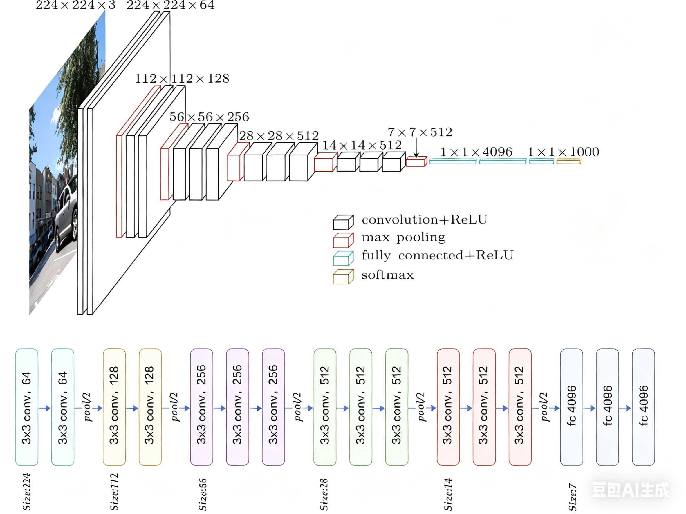
VGG16是最常用和最經典的VGG變體之一。數字“16”指的是網絡中包含權重參數的層數,即13個卷積層 + 3個全連接層 = 16層。池化層和激活層不計入此數。
具體參數如下:
| 階段 | 層類型 | 輸出尺寸 (C x H x W) | 參數配置 (核大小/步長/填充) | 輸出通道數 | 備注 |
|---|---|---|---|---|---|
| 輸入 | Input Image | 3 x 224 x 224 | - | - | 假設輸入圖像尺寸為224x224 |
| Block 1 | Conv3-64 | 64 x 224 x 224 | 3x3 / 1 / 1 | 64 | |
| Conv3-64 | 64 x 224 x 224 | 3x3 / 1 / 1 | 64 | ||
| MaxPool | 64 x 112 x 112 | 2x2 / 2 | - | 尺寸減半 | |
| Block 2 | Conv3-128 | 128 x 112 x 112 | 3x3 / 1 / 1 | 128 | |
| Conv3-128 | 128 x 112 x 112 | 3x3 / 1 / 1 | 128 | ||
| MaxPool | 128 x 56 x 56 | 2x2 / 2 | - | 尺寸減半 | |
| Block 3 | Conv3-256 | 256 x 56 x 56 | 3x3 / 1 / 1 | 256 | |
| Conv3-256 | 256 x 56 x 56 | 3x3 / 1 / 1 | 256 | ||
| Conv3-256 | 256 x 56 x 56 | 3x3 / 1 / 1 | 256 | ||
| MaxPool | 256 x 28 x 28 | 2x2 / 2 | - | 尺寸減半 | |
| Block 4 | Conv3-512 | 512 x 28 x 28 | 3x3 / 1 / 1 | 512 | |
| Conv3-512 | 512 x 28 x 28 | 3x3 / 1 / 1 | 512 | ||
| Conv3-512 | 512 x 28 x 28 | 3x3 / 1 / 1 | 512 | ||
| MaxPool | 512 x 14 x 14 | 2x2 / 2 | - | 尺寸減半 | |
| Block 5 | Conv3-512 | 512 x 14 x 14 | 3x3 / 1 / 1 | 512 | |
| Conv3-512 | 512 x 14 x 14 | 3x3 / 1 / 1 | 512 | ||
| Conv3-512 | 512 x 14 x 14 | 3x3 / 1 / 1 | 512 | ||
| MaxPool | 512 x 7 x 7 | 2x2 / 2 | - | 尺寸減半 | |
| FC | Flatten | 1 x 25088 | - | - | 將特征圖展平為一維向量 |
| FC-4096 | 4096 | - | 4096 | 全連接層1 | |
| FC-4096 | 4096 | - | 4096 | 全連接層2 | |
| FC-1000 | 1000 | - | 1000 | 輸出層 (Softmax) |
關鍵點說明
-
卷積塊(Conv Block): 每個Block由連續的2-3個3x3卷積層組成,通道數在Block內保持不變(如Block1都是64通道),在Block之間通過池化層后翻倍(64->128->256->512->512)。Block5的通道數沒有繼續翻倍,保持512。
-
池化層(MaxPool): 位于每個卷積塊之后,負責降低空間維度(H, W減半),增加感受野,并一定程度上提供平移不變性。
-
全連接層(FC):
-
在最后一個池化層(輸出尺寸為
512 x 7 x 7)之后,將特征圖展平(Flat) 成一個長度為512 * 7 * 7 = 25088的一維向量。 -
然后依次通過兩個4096維的全連接層(通常使用ReLU激活和Dropout防止過擬合)。
-
最后是一個1000維的全連接層(對應ImageNet的1000類),使用Softmax函數輸出每個類別的預測概率。
-
-
激活函數: 所有卷積層和全連接層(除最后一層)之后都使用ReLU激活函數,引入非線性。
-
參數量: VGG16的總參數量約為138 million (1.38億)。其中,絕大部分參數(約90%)集中在最后的三個全連接層(FC-4096: ~102M, FC-4096: ~102M, FC-1000: ~4M)。卷積層的參數量相對較少(約27M)。
3 VGG的優缺點
3.1 核心優點
-
設計簡潔統一,易于理解與實現
-
規則化結構:所有卷積層均使用 3×3核(除少量1×1卷積),所有池化層均使用 2×2最大池化,模塊化設計清晰。
-
配置單一:卷積層參數固定(
stride=1, padding=1),池化層參數固定(stride=2),無需復雜調參。 -
代碼復用性高:相同結構的卷積塊可循環實現,降低工程復雜度。
-
-
深度網絡性能的強力證明
-
深度提升效果顯著:通過對比VGG11(11層)到VGG19(19層),證明增加深度能持續提升精度(ImageNet Top-5錯誤率從10.4%降至7.3%)。
-
小卷積核的優越性:
在相同感受野的情況下,堆疊小卷積核相比使用大卷積核具有更多的激活函數、更豐富的特征,更強的辨別能力。卷積后都伴有激活函數,可使決策函數更加具有辨別能力;此外,3x3比7x7就足以捕獲細節特征的變化:3x3的9個格子,最中間的格子是一個感受野中心,可以捕獲上下左右以及斜對角的特征變化;3個3x3堆疊近似一個7x7,網絡深了兩層且多出了兩個非線性ReLU函數,網絡容量更大,對于不同類別的區分能力更強。
-
-
強大的特征提取能力
-
分層特征學習:
-
淺層(Block1-2)學習邊緣、紋理等低級特征。
-
中層(Block3-4)學習物體部件等中級特征。
-
深層(Block5-FC)學習語義等高級特征。
-
-
特征泛用性強:預訓練模型(尤其VGG16/19)的卷積層特征被廣泛用于遷移學習(如目標檢測、圖像分割)。
-
3.2 顯著缺點
-
參數量巨大,計算成本高昂
-
參數分布:
層類型 參數量(VGG16) 占比 卷積層 ≈14.7M 10.6% 全連接層 ≈123.6M 89.4% 總計 ≈138.3M 100% -
計算開銷:
-
訓練需大量GPU資源(如VGG19訓練耗時約2-3周,單卡V100)。
-
推理速度慢(224×224圖像在V100上約100ms,遠低于MobileNet)。
-
-
-
全連接層(FC)的致命缺陷
-
參數冗余:FC層占90%參數,但貢獻有限(后續研究表明可用全局平均池化替代)。
-
空間限制:FC層要求固定輸入尺寸(如224×224),需對圖像裁剪/縮放,可能丟失信息。
-
過擬合風險:FC層參數多,在小型數據集上易過擬合(需強正則化如Dropout)。
-
-
內存與存儲瓶頸
-
顯存占用高:訓練時需存儲大量中間特征圖(如Block5輸出512×7×7,需≈10MB顯存)。
-
模型體積大:VGG16模型文件超500MB,不適合移動端/嵌入式部署。
-
-
用多個 3×3卷積代替大卷積,會增加網絡深度,深度過大可能帶來梯度消失或梯度爆炸問題。
-
解決方案:
-
使用 Batch Normalization(BN) 進行歸一化。
-
采用 ResNet 殘差連接,保證梯度有效傳播。
-
-
-
結構僵化,缺乏創新性
-
無多尺度處理:未采用Inception的多分支結構或ResNet的殘差連接,特征融合能力弱。
-
通道設計保守:通道數僅按2倍增長(64→128→256→512),未探索更高效的通道分配策略。
-
總結:VGG是深度學習史上的“功勛模型”,其簡潔設計和深度探索為后續發展鋪平道路。盡管因參數冗余、計算低效逐漸退出主流,但其特征提取能力和設計思想仍具重要參考價值。在資源充足或需要強特征的任務中,VGG仍是可靠選擇;但對效率敏感的場景,需選擇更現代的輕量架構。
4 基于Pytorch實現
以下項目實現了 VGG 網絡,并在 CIFAR10 上驗證了該網絡的有效性,項目目錄如下:
VGG_CIFAR10/│├── model/ ? ? ? ? ? ? ? ? ?# 存放模型定義│ ? ├── __init__.py│ ? └── VGG.py ? ? ? ? ? ? ?# VGG模型定義│├── data/ ? ? ? ? ? ? ? ? ? # 存放數據集(CIFAR-10會自動下載)│├── utils/ ? ? ? ? ? ? ? ? ?# 工具函數│ ? ├── __init__.py│ ? ├── transforms.py ? ? ? # 數據預處理│ ? └── visualization.py ? ? # 可視化工具│├── train.py ? ? ? ? ? ? ? ?# 訓練腳本├── test.py ? ? ? ? ? ? ? ? # 測試腳本└── config.py ? ? ? ? ? ? ? # 配置文件配置文件
?# config.pyimport torch?# 訓練參數class Config:# 數據參數data_dir = './data'batch_size = 128num_workers = 4?# 模型參數num_classes = 10model_name = 'vgg16'?# 訓練參數num_epochs = 50learning_rate = 0.01momentum = 0.9weight_decay = 5e-4lr_step_size = 30lr_gamma = 0.1?# 其他device = 'cuda' if torch.cuda.is_available() else 'cpu'save_path = './checkpoints/'log_interval = 100模型定義
?
# VGG.pyimport torchimport torch.nn as nn??class VGG(nn.Module):def __init__(self, num_classes=10, init_weights=True):super(VGG, self).__init__()?# 特征提取部分(卷積層)self.features = nn.Sequential(# Block 1nn.Conv2d(3, 64, kernel_size=3, padding=1),nn.BatchNorm2d(64), ?# 添加批歸一化nn.ReLU(inplace=True),nn.Conv2d(64, 64, kernel_size=3, padding=1),nn.BatchNorm2d(64),nn.ReLU(inplace=True),nn.MaxPool2d(kernel_size=2, stride=2),?# Block 2nn.Conv2d(64, 128, kernel_size=3, padding=1),nn.BatchNorm2d(128),nn.ReLU(inplace=True),nn.Conv2d(128, 128, kernel_size=3, padding=1),nn.BatchNorm2d(128),nn.ReLU(inplace=True),nn.MaxPool2d(kernel_size=2, stride=2),?# Block 3nn.Conv2d(128, 256, kernel_size=3, padding=1),nn.BatchNorm2d(256),nn.ReLU(inplace=True),nn.Conv2d(256, 256, kernel_size=3, padding=1),nn.BatchNorm2d(256),nn.ReLU(inplace=True),nn.Conv2d(256, 256, kernel_size=3, padding=1),nn.BatchNorm2d(256),nn.ReLU(inplace=True),nn.MaxPool2d(kernel_size=2, stride=2),?# Block 4nn.Conv2d(256, 512, kernel_size=3, padding=1),nn.BatchNorm2d(512),nn.ReLU(inplace=True),nn.Conv2d(512, 512, kernel_size=3, padding=1),nn.BatchNorm2d(512),nn.ReLU(inplace=True),nn.Conv2d(512, 512, kernel_size=3, padding=1),nn.BatchNorm2d(512),nn.ReLU(inplace=True),nn.MaxPool2d(kernel_size=2, stride=2),?# Block 5nn.Conv2d(512, 512, kernel_size=3, padding=1),nn.BatchNorm2d(512),nn.ReLU(inplace=True),nn.Conv2d(512, 512, kernel_size=3, padding=1),nn.BatchNorm2d(512),nn.ReLU(inplace=True),nn.Conv2d(512, 512, kernel_size=3, padding=1),nn.BatchNorm2d(512),nn.ReLU(inplace=True),nn.MaxPool2d(kernel_size=2, stride=2))?# 分類器部分(全連接層)self.avgpool = nn.AdaptiveAvgPool2d((7, 7))self.classifier = nn.Sequential(nn.Linear(512 * 7 * 7, 4096),nn.ReLU(inplace=True),nn.Dropout(0.5), ?# 增加Dropout率nn.Linear(4096, 4096),nn.ReLU(inplace=True),nn.Dropout(0.5),nn.Linear(4096, num_classes))?if init_weights:self._initialize_weights()?def forward(self, x):x = self.features(x)x = self.avgpool(x)x = torch.flatten(x, 1)x = self.classifier(x)return x?def _initialize_weights(self):for m in self.modules():if isinstance(m, nn.Conv2d):nn.init.kaiming_normal_(m.weight, mode='fan_out', nonlinearity='relu')if m.bias is not None:nn.init.constant_(m.bias, 0)elif isinstance(m, nn.BatchNorm2d):nn.init.constant_(m.weight, 1)nn.init.constant_(m.bias, 0)elif isinstance(m, nn.Linear):nn.init.normal_(m.weight, 0, 0.01)nn.init.constant_(m.bias, 0)??def vgg16(num_classes=10):return VGG(num_classes=num_classes)工具函數
?# transforms.pyimport torchvision.transforms as transforms?def get_train_transform():return transforms.Compose([transforms.RandomCrop(32, padding=4),transforms.RandomHorizontalFlip(),transforms.RandomRotation(15), ?# 添加隨機旋轉transforms.ColorJitter(brightness=0.2, contrast=0.2, saturation=0.2), ?# 顏色抖動transforms.ToTensor(),transforms.Normalize((0.4914, 0.4822, 0.4465), (0.2023, 0.1994, 0.2010)),])?def get_test_transform():return transforms.Compose([transforms.ToTensor(),transforms.Normalize((0.4914, 0.4822, 0.4465), (0.2023, 0.1994, 0.2010)),])?# visualization.pyimport matplotlib.pyplot as pltimport numpy as npimport torch??'''用于訓練可視化'''def plot_results(train_losses, train_accs, test_losses, test_accs):plt.figure(figsize=(12, 4))?# 繪制損失曲線plt.subplot(1, 2, 1)plt.plot(train_losses, label='Train Loss')plt.plot(test_losses, label='Test Loss')plt.xlabel('Epoch')plt.ylabel('Loss')plt.legend()plt.title('Training and Test Loss')?# 繪制準確率曲線plt.subplot(1, 2, 2)plt.plot(train_accs, label='Train Accuracy')plt.plot(test_accs, label='Test Accuracy')plt.xlabel('Epoch')plt.ylabel('Accuracy')plt.legend()plt.title('Training and Test Accuracy')?plt.tight_layout()plt.savefig('results.png')plt.show()??'''用于測試可視化'''def visualize_predictions(model, device, test_loader, classes, num_samples=8):# 獲取一批測試數據dataiter = iter(test_loader)images, labels = next(dataiter)?# 選擇前num_samples個樣本images = images[:num_samples]labels = labels[:num_samples]?# 將圖像移至設備images = images.to(device)?# 獲取模型預測outputs = model(images)_, predicted = torch.max(outputs, 1)?# 將預測和標簽移回CPUpredicted = predicted.cpu().numpy()labels = labels.numpy()?# 顯示圖像plt.figure(figsize=(12, 6))for i in range(num_samples):plt.subplot(2, 4, i + 1)# 反歸一化img = images[i].cpu().numpy().transpose(1, 2, 0)mean = np.array([0.4914, 0.4822, 0.4465])std = np.array([0.2023, 0.1994, 0.2010])img = std * img + meanimg = np.clip(img, 0, 1)plt.imshow(img)plt.title(f"True: {classes[labels[i]]}\nPred: {classes[predicted[i]]}")plt.axis('off')plt.tight_layout()plt.savefig('predictions.png')plt.show()模型訓練
?# train.pyimport torchimport torch.optim as optimimport torch.nn.functional as Ffrom torch.utils.data import DataLoaderfrom torchvision import datasetsimport osimport timefrom tqdm import tqdm?from model.VGG import vgg16from utils.transforms import get_train_transform, get_test_transformfrom utils.visualization import plot_resultsfrom config import Config??def train(model, device, train_loader, optimizer, epoch, config):model.train()running_loss = 0.0correct = 0total = 0?progress_bar = tqdm(train_loader, desc=f'Epoch {epoch}/{config.num_epochs}')for batch_idx, (inputs, targets) in enumerate(progress_bar):inputs, targets = inputs.to(device), targets.to(device)?# 前向傳播outputs = model(inputs)loss = F.cross_entropy(outputs, targets)?# 反向傳播與優化optimizer.zero_grad()loss.backward()optimizer.step()?# 統計信息running_loss += loss.item()_, predicted = outputs.max(1)total += targets.size(0)correct += predicted.eq(targets).sum().item()?# 更新進度條progress_bar.set_postfix({'Loss': running_loss / (batch_idx + 1),'Acc': 100. * correct / total})?train_loss = running_loss / len(train_loader)train_acc = 100. * correct / totalreturn train_loss, train_acc??def test(model, device, test_loader):model.eval()test_loss = 0correct = 0total = 0?with torch.no_grad():for inputs, targets in test_loader:inputs, targets = inputs.to(device), targets.to(device)outputs = model(inputs)test_loss += F.cross_entropy(outputs, targets, reduction='sum').item()_, predicted = outputs.max(1)total += targets.size(0)correct += predicted.eq(targets).sum().item()?test_loss /= len(test_loader.dataset)test_acc = 100. * correct / totalreturn test_loss, test_acc??def main():config = Config()?# 創建保存目錄os.makedirs(config.save_path, exist_ok=True)?# 加載數據集train_set = datasets.CIFAR10(root=config.data_dir, train=True, download=True, transform=get_train_transform())test_set = datasets.CIFAR10(root=config.data_dir, train=False, download=True, transform=get_test_transform())?train_loader = DataLoader(train_set, batch_size=config.batch_size, shuffle=True, num_workers=config.num_workers)test_loader = DataLoader(test_set, batch_size=config.batch_size, shuffle=False, num_workers=config.num_workers)?# 創建模型model = vgg16(num_classes=config.num_classes).to(config.device)?# 打印模型結構print(model)?# 定義優化器和損失函數optimizer = optim.SGD(model.parameters(),lr=config.learning_rate,momentum=config.momentum,weight_decay=config.weight_decay)scheduler = optim.lr_scheduler.StepLR(optimizer, step_size=config.lr_step_size, gamma=config.lr_gamma)?# 訓練記錄train_losses = []train_accs = []test_losses = []test_accs = []best_acc = 0.0?# 訓練循環for epoch in range(1, config.num_epochs + 1):start_time = time.time()?# 訓練train_loss, train_acc = train(model, config.device, train_loader, optimizer, epoch, config)?# 測試test_loss, test_acc = test(model, config.device, test_loader)?# 學習率調整scheduler.step()?# 記錄train_losses.append(train_loss)train_accs.append(train_acc)test_losses.append(test_loss)test_accs.append(test_acc)?# 保存最佳模型if test_acc > best_acc:best_acc = test_acctorch.save(model.state_dict(), os.path.join(config.save_path, 'best_model.pth'))?# 打印信息elapsed_time = time.time() - start_timeprint(f'Epoch {epoch}/{config.num_epochs} - Time: {elapsed_time:.2f}s')print(f'Train Loss: {train_loss:.4f}, Train Acc: {train_acc:.2f}%')print(f'Test Loss: {test_loss:.4f}, Test Acc: {test_acc:.2f}%')print(f'Best Test Acc: {best_acc:.2f}%\n')?# 繪制結果plot_results(train_losses, train_accs, test_losses, test_accs)?print(f'Training completed. Best test accuracy: {best_acc:.2f}%')??if __name__ == '__main__':main()模型測試
# test.py?
import torchfrom torch.utils.data import DataLoaderfrom torchvision import datasetsimport os?from model.VGG import vgg16from utils.transforms import get_test_transformfrom utils.visualization import visualize_predictionsfrom config import Config??def main():config = Config()?# 加載測試數據集test_set = datasets.CIFAR10(root=config.data_dir, train=False, download=True, transform=get_test_transform())test_loader = DataLoader(test_set, batch_size=config.batch_size, shuffle=False, num_workers=config.num_workers)?# 加載模型model = vgg16(num_classes=config.num_classes).to(config.device)model.load_state_dict(torch.load(os.path.join(config.save_path, 'best_model.pth')))model.eval()?# 類別標簽classes = ('plane', 'car', 'bird', 'cat', 'deer','dog', 'frog', 'horse', 'ship', 'truck')?# 可視化預測結果visualize_predictions(model, config.device, test_loader, classes)??if __name__ == '__main__':main()

)


)


 的兼容性問題)


