一、無監督學習(Unsupervised Learning)

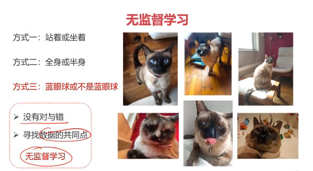
機器學習的一種方法,沒有給定事先標記過的訓練示例,自動對輸入的數據進行分類或分群。
優點:
- 算法不受監督信息(偏見)的約束,可能考慮到新的信息
- 不需要標簽數據,極大程度擴大數據樣本
主要應用:聚類分析、關聯規則、維度縮減
應用最廣:聚類分析(clustering)
二、聚類分析
聚類分析又稱為群分析,根據對象某些屬性的相似度,將其自動化分為不同的類別。

常用的聚類算法
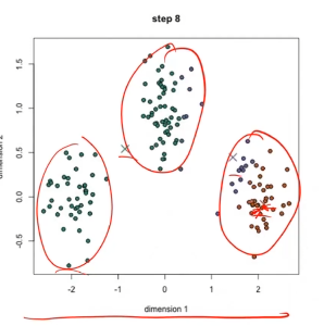
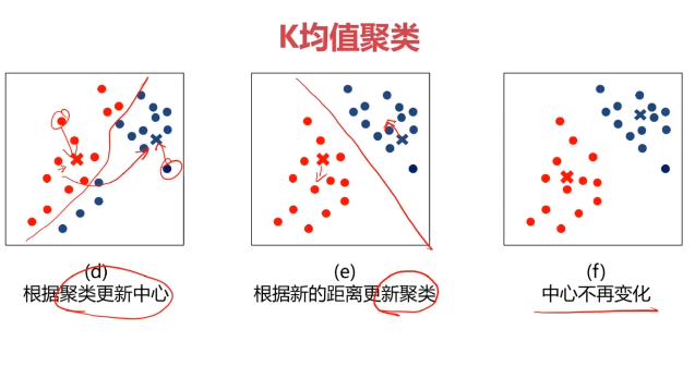
1、KMeans聚類
- 根據數據與中心點距離劃分類別
- 基于類別數據更新中心點
- 重復過程直到收斂
特點:
1、實現簡單,收斂快
2、需要指定類別數量
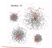
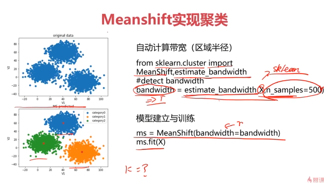
2、均值漂移聚類(Meanshift)
- 在中心點一定區域檢索數據點
- 更新中心
- 重復流程到中心點穩定
特點:
1、自動發現類別數量,不需要人工選擇
2、需要選擇區域半徑
3、DBSCAN算法(基于密度的空間聚類算法)
- 基于區域點密度篩選有效數據
- 基于有效數據向周邊擴張,直到沒有新點加入

特點:
1、過濾噪音數據
2、不需要人為選擇類別數量
3、數據密度不同時影響結果
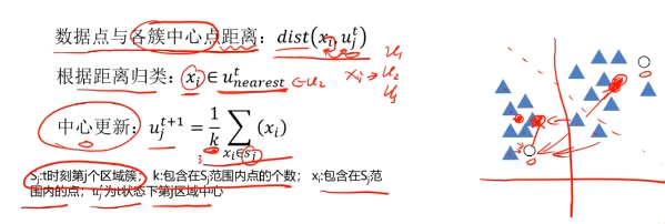
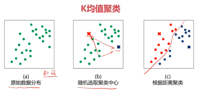
4、什么是K均值聚類?(KMeans Analysis)
K-均值算法:以空間中k個點為中心進行聚類,對最靠近他們的對象歸類,是聚類算法中最為基礎但也最為重要的算法。

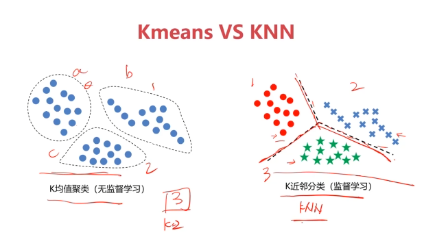
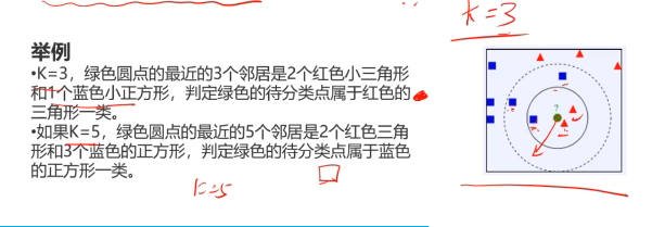
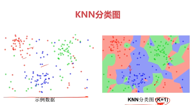
5、K近鄰分類模型(KNN)
給定一個訓練數據集,對新的輸入實例,在訓練數據集中找到與該實例最鄰近的K個實例(也就是上面所說的K個鄰居),這K個實例的多數屬于某個類,就把該輸入實例分類到這個類中
- 最簡單的機器學習算法之一
5、均值漂移聚類(Meanshift)
均值漂移算法:一種基于密度梯度上升的聚類算法(沿著密度上升方向尋找聚類中心點)
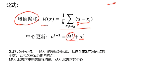
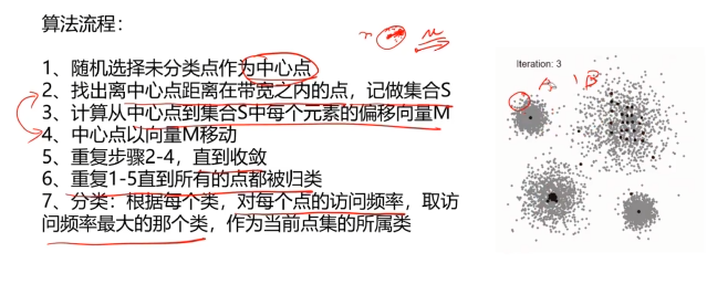
6、實現過程
三、使用Kmeans算法實現2D數據自動聚類
#使用Kmeans算法實現2D數據自動聚類,使用數據集kmeans_data.csv
#加載數據
import pandas as pd
import numpy as np
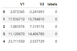
data = pd.read_csv('kmeans_data.csv')
data.head()
#賦值x y
x = data.drop('labels',axis=1)
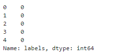
y = data.loc[:,'labels']
y.head()
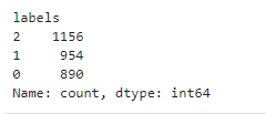
#查看labels有多少類別
pd.Series.value_counts(y)
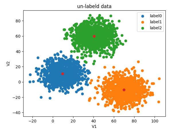
#畫圖
from matplotlib import pyplot as plt
fig1 = plt.figure()
plt.scatter(x.loc[:,'V1'],x.loc[:,'V2'])
plt.title('un-labeld data')
plt.xlabel('V1')
plt.ylabel('V2')
plt.show()
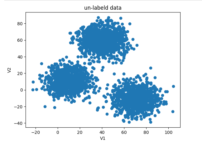
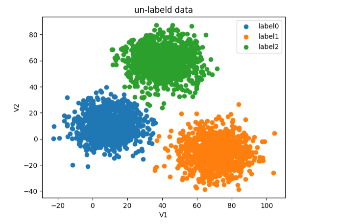
fig2 = plt.figure()
label0 = plt.scatter(x.loc[:,'V1'][y==0],x.loc[:,'V2'][y==0])
label1 = plt.scatter(x.loc[:,'V1'][y==1],x.loc[:,'V2'][y==1])
label2 = plt.scatter(x.loc[:,'V1'][y==2],x.loc[:,'V2'][y==2])
plt.title('un-labeld data')
plt.xlabel('V1')
plt.ylabel('V2')
plt.legend((label0,label1,label2),('label0','label1','label2'))
plt.show()
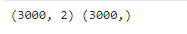
#查看x y維度
print(x.shape,y.shape)
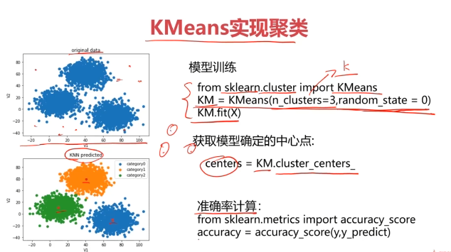
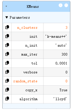
#創建Kmeans模型
from sklearn.cluster import KMeans
KM = KMeans(n_clusters=3,random_state=0)
KM.fit(x)
#聚類的中心點
centers = KM.cluster_centers_
fig3 = plt.figure()
label0 = plt.scatter(x.loc[:,'V1'][y==0],x.loc[:,'V2'][y==0])
label1 = plt.scatter(x.loc[:,'V1'][y==1],x.loc[:,'V2'][y==1])
label2 = plt.scatter(x.loc[:,'V1'][y==2],x.loc[:,'V2'][y==2])
plt.scatter(centers[:,0],centers[:,1])
plt.title('un-labeld data')
plt.xlabel('V1')
plt.ylabel('V2')
plt.legend((label0,label1,label2),('label0','label1','label2'))
plt.show()
#測試新數據V1=80,V2=60
x_test = pd.DataFrame([[80,60]],columns=['V1','V2'])
y_predict_test = KM.predict(x_test)
print(y_predict_test)
#計算準確率
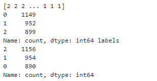
y_predict = KM.predict(x)
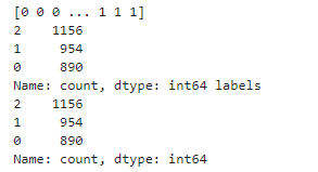
print(y_predict)
print(pd.Series.value_counts(y_predict),pd.Series.value_counts(y))
from sklearn.metrics import accuracy_score
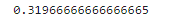
accuracy = accuracy_score(y,y_predict)
print(accuracy)
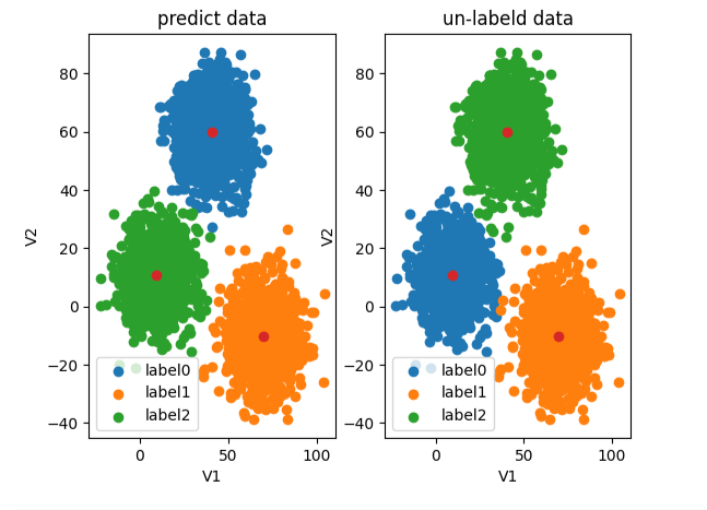
#可視化數據
fig4 = plt.subplot(121)
label0 = plt.scatter(x.loc[:,'V1'][y_predict==0],x.loc[:,'V2'][y_predict==0])
label1 = plt.scatter(x.loc[:,'V1'][y_predict==1],x.loc[:,'V2'][y_predict==1])
label2 = plt.scatter(x.loc[:,'V1'][y_predict==2],x.loc[:,'V2'][y_predict==2])
plt.scatter(centers[:,0],centers[:,1])
plt.title('predict data')
plt.xlabel('V1')
plt.ylabel('V2')
plt.legend((label0,label1,label2),('label0','label1','label2'))fig5 = plt.subplot(122)
label0 = plt.scatter(x.loc[:,'V1'][y==0],x.loc[:,'V2'][y==0])
label1 = plt.scatter(x.loc[:,'V1'][y==1],x.loc[:,'V2'][y==1])
label2 = plt.scatter(x.loc[:,'V1'][y==2],x.loc[:,'V2'][y==2])
plt.scatter(centers[:,0],centers[:,1])
plt.title('un-labeld data')
plt.xlabel('V1')
plt.ylabel('V2')
plt.legend((label0,label1,label2),('label0','label1','label2'))
plt.show()
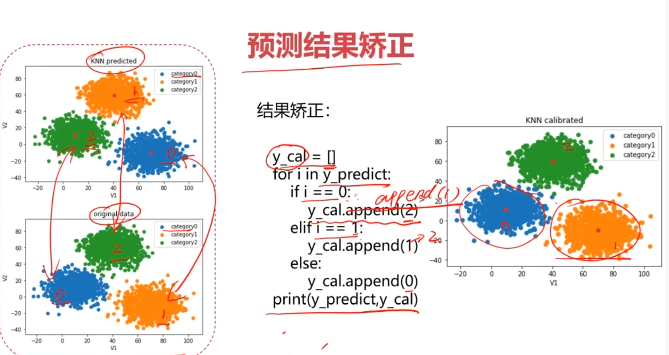
#校正結果
y_corrected = []
for i in y_predict:if i==0:y_corrected.append(2)elif i==1:y_corrected.append(1)else:y_corrected.append(0)print(pd.Series.value_counts(y_corrected),pd.Series.value_counts(y))
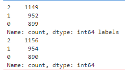
#打印準確率
print(accuracy_score(y,y_corrected))
y_corrected = np.array(y_corrected)
print(type(y_corrected))
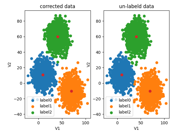
#可視化數據
fig6 = plt.subplot(121)
label0 = plt.scatter(x.loc[:,'V1'][y_corrected==0],x.loc[:,'V2'][y_corrected==0])
label1 = plt.scatter(x.loc[:,'V1'][y_corrected==1],x.loc[:,'V2'][y_corrected==1])
label2 = plt.scatter(x.loc[:,'V1'][y_corrected==2],x.loc[:,'V2'][y_corrected==2])
plt.scatter(centers[:,0],centers[:,1])
plt.title('corrected data')
plt.xlabel('V1')
plt.ylabel('V2')
plt.legend((label0,label1,label2),('label0','label1','label2'))fig7 = plt.subplot(122)
label0 = plt.scatter(x.loc[:,'V1'][y==0],x.loc[:,'V2'][y==0])
label1 = plt.scatter(x.loc[:,'V1'][y==1],x.loc[:,'V2'][y==1])
label2 = plt.scatter(x.loc[:,'V1'][y==2],x.loc[:,'V2'][y==2])
plt.scatter(centers[:,0],centers[:,1])
plt.title('un-labeld data')
plt.xlabel('V1')
plt.ylabel('V2')
plt.legend((label0,label1,label2),('label0','label1','label2'))
plt.show()
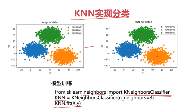
四、使用監督學習KNN算法
from sklearn.neighbors import KNeighborsClassifier
KNN = KNeighborsClassifier(n_neighbors=3)
KNN.fit(x,y)

#測試新數據V1=80,V2=60
x_test = pd.DataFrame([[80,60]],columns=['V1','V2'])
y_predict_test = KNN.predict(x_test)
print(y_predict_test)

#計算準確率
y_knn_predict = KNN.predict(x)
print(y_knn_predict)
print(pd.Series.value_counts(y_knn_predict),pd.Series.value_counts(y))
from sklearn.metrics import accuracy_score
accuracy = accuracy_score(y,y_knn_predict)
print(accuracy)

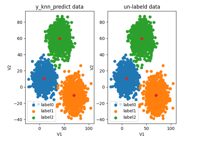
#可視化數據
fig8 = plt.subplot(121)
label0 = plt.scatter(x.loc[:,'V1'][y_knn_predict==0],x.loc[:,'V2'][y_knn_predict==0])
label1 = plt.scatter(x.loc[:,'V1'][y_knn_predict==1],x.loc[:,'V2'][y_knn_predict==1])
label2 = plt.scatter(x.loc[:,'V1'][y_knn_predict==2],x.loc[:,'V2'][y_knn_predict==2])
plt.scatter(centers[:,0],centers[:,1])
plt.title('y_knn_predict data')
plt.xlabel('V1')
plt.ylabel('V2')
plt.legend((label0,label1,label2),('label0','label1','label2'))fig9 = plt.subplot(122)
label0 = plt.scatter(x.loc[:,'V1'][y==0],x.loc[:,'V2'][y==0])
label1 = plt.scatter(x.loc[:,'V1'][y==1],x.loc[:,'V2'][y==1])
label2 = plt.scatter(x.loc[:,'V1'][y==2],x.loc[:,'V2'][y==2])
plt.scatter(centers[:,0],centers[:,1])
plt.title('un-labeld data')
plt.xlabel('V1')
plt.ylabel('V2')
plt.legend((label0,label1,label2),('label0','label1','label2'))
plt.show()
五、使用 Meanshift 算法
#使用 Meanshift 算法
from sklearn.cluster import MeanShift,estimate_bandwidth
#獲取范圍帶寬、半徑
bw = estimate_bandwidth(x,n_samples=500)
print(bw)

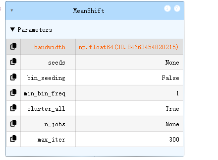
#創建模型,訓練模型
ms = MeanShift(bandwidth=bw)
ms.fit(x)
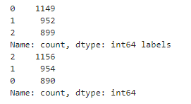
y_predict_meanshift = ms.predict(x)
print(pd.Series.value_counts(y_predict_meanshift),pd.Series.value_counts(y))
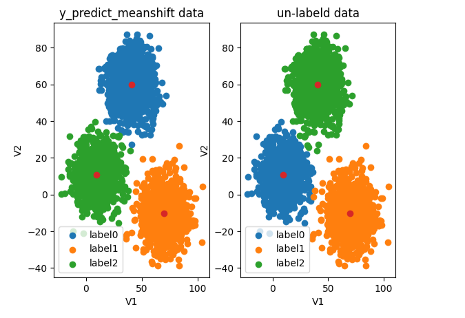
#可視化數據
fig10 = plt.subplot(121)
label0 = plt.scatter(x.loc[:,'V1'][y_predict_meanshift==0],x.loc[:,'V2'][y_predict_meanshift==0])
label1 = plt.scatter(x.loc[:,'V1'][y_predict_meanshift==1],x.loc[:,'V2'][y_predict_meanshift==1])
label2 = plt.scatter(x.loc[:,'V1'][y_predict_meanshift==2],x.loc[:,'V2'][y_predict_meanshift==2])
plt.scatter(centers[:,0],centers[:,1])
plt.title('y_predict_meanshift data')
plt.xlabel('V1')
plt.ylabel('V2')
plt.legend((label0,label1,label2),('label0','label1','label2'))fig11 = plt.subplot(122)
label0 = plt.scatter(x.loc[:,'V1'][y==0],x.loc[:,'V2'][y==0])
label1 = plt.scatter(x.loc[:,'V1'][y==1],x.loc[:,'V2'][y==1])
label2 = plt.scatter(x.loc[:,'V1'][y==2],x.loc[:,'V2'][y==2])
plt.scatter(centers[:,0],centers[:,1])
plt.title('un-labeld data')
plt.xlabel('V1')
plt.ylabel('V2')
plt.legend((label0,label1,label2),('label0','label1','label2'))
plt.show()
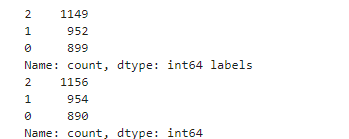
#校正結果
y_corrected = []
for i in y_predict_meanshift:if i==0:y_corrected.append(2)elif i==1:y_corrected.append(1)else:y_corrected.append(0)print(pd.Series.value_counts(y_corrected),pd.Series.value_counts(y))
y_corrected = np.array(y_corrected)
print(type(y_corrected))
#可視化數據
fig12 = plt.subplot(121)
label0 = plt.scatter(x.loc[:,'V1'][y_corrected==0],x.loc[:,'V2'][y_corrected==0])
label1 = plt.scatter(x.loc[:,'V1'][y_corrected==1],x.loc[:,'V2'][y_corrected==1])
label2 = plt.scatter(x.loc[:,'V1'][y_corrected==2],x.loc[:,'V2'][y_corrected==2])
plt.scatter(centers[:,0],centers[:,1])
plt.title('corrected data')
plt.xlabel('V1')
plt.ylabel('V2')
plt.legend((label0,label1,label2),('label0','label1','label2'))fig13 = plt.subplot(122)
label0 = plt.scatter(x.loc[:,'V1'][y==0],x.loc[:,'V2'][y==0])
label1 = plt.scatter(x.loc[:,'V1'][y==1],x.loc[:,'V2'][y==1])
label2 = plt.scatter(x.loc[:,'V1'][y==2],x.loc[:,'V2'][y==2])
plt.scatter(centers[:,0],centers[:,1])
plt.title('un-labeld data')
plt.xlabel('V1')
plt.ylabel('V2')
plt.legend((label0,label1,label2),('label0','label1','label2'))
plt.show()

)


)


)


李宏毅2025大模型-作業4)
