這一節告訴你如何用TensorFlow實現全連接網絡。
安裝 DeepChem
這一節,你將使用DeepChem 機器學習工具鏈進行實驗在網上可以找到 DeepChem詳細安裝指導。
Tox21 Dataset
作為我們的建模案例研究,我們使用化學數據庫。毒理學家很感興趣于用機器學習來預測化學物是有毒。這個任務很復雜,因為令天的科學對代謝過程了解得很少。但是,生物學家和化學家用有限的實驗來提示毒性。如果一個化學物命中這個實驗之一,它很可能對人類有毒。但是這些實驗成本很高。所以數據學家構建機器學習模型來預測新化合物的結果。
一個重要的毒理學數據集是Tox21。我們分析 Tox21里的其中一個數據集。這個數據集有 10,000個化學物與雄激素受體的相互作有用。數據科學家需要預測新化合物是否與雄激素受體有相互作用。處理數據集很有技巧,所有要用DeepChem里的MoleculeNet 數據集。 Each molecule in Tox21里的分子被DeepChem處理為長度為1024的位-向量。簡單的調用DeepChem來加載數據集 (Example 4-1).
Example 4-1. Load the Tox21 dataset
import deepchem as dc
_, (train, valid, test), _ = dc.molnet.load_tox21()
train_X, train_y, train_w = train.X, train.y, train.w
valid_X, valid_y, valid_w = valid.X, valid.y, valid.w
test_X, test_y, test_w = test.X, test.y, test.w
這里 X是處理過的特征向量, y 是標簽,? w 是權重。標簽是 1/0 表示是否與雄激素交互。 Tox21 存貯不平衡數據集,正樣本數少于負樣本數。所有的變量為NumPy 數組。Tox21有很多數據集我們不需要在這里分析,所以我們要去除這相關的數據集的標簽。 (Example 4-2).
Example 4-2. Remove extra datasets from Tox21
# Remove extra tasks
train_y = train_y[:, 0]
valid_y = valid_y[:, 0]
test_y = test_y[:, 0]
train_w = train_w[:, 0]
valid_w = valid_w[:, 0]
test_w = test_w[:, 0]
接收Minibatches為Placeholders
(Example 4-3).
Example 4-3. Defining placeholders that accept minibatches of different sizes
d = 1024
with tf.name_scope("placeholders"):
x = tf.placeholder(tf.float32, (None, d))
y = tf.placeholder(tf.float32, (None,))
Note d is 1024, the dimensionality of our feature vectors.
實現隱藏層
?Example 4-4.
Example 4-4. Defining a hidden layer
with tf.name_scope("hidden-layer"):
W = tf.Variable(tf.random_normal((d, n_hidden)))
b = tf.Variable(tf.random_normal((n_hidden,)))
x_hidden = tf.nn.relu(tf.matmul(x, W) + b)
我們使用 tf.nn.relu激活函數。其它代碼與邏輯回歸的代碼相似。
?Example 4-5.
Example 4-5. Defining the fully connected architecture
with tf.name_scope("placeholders"):
x = tf.placeholder(tf.float32, (None, d))
y = tf.placeholder(tf.float32, (None,))
with tf.name_scope("hidden-layer"):
W = tf.Variable(tf.random_normal((d, n_hidden)))
b = tf.Variable(tf.random_normal((n_hidden,)))
x_hidden = tf.nn.relu(tf.matmul(x, W) + b)
with tf.name_scope("output"):
W = tf.Variable(tf.random_normal((n_hidden, 1)))
b = tf.Variable(tf.random_normal((1,)))
y_logit = tf.matmul(x_hidden, W) + b
# the sigmoid gives the class probability of 1
y_one_prob = tf.sigmoid(y_logit)
# Rounding P(y=1) will give the correct prediction.
y_pred = tf.round(y_one_prob)
with tf.name_scope("loss"):
# Compute the cross-entropy term for each datapoint
y_expand = tf.expand_dims(y, 1)
entropy = tf.nn.sigmoid_cross_entropy_with_logits(logits=y_logit, labels=y_expand)
# Sum all contributions
l = tf.reduce_sum(entropy)
with tf.name_scope("optim"):
train_op = tf.train.AdamOptimizer(learning_rate).minimize(l)
with tf.name_scope("summaries"):
tf.summary.scalar("loss", l)
merged = tf.summary.merge_all()
添加Dropout到隱藏層
TensorFlow 使用tf.nn.dropout(x, keep_prob)為我們實現dropout,其中 keep_prob 是節點保留的概率。記住在訓練時打開dropout,預測時關閉dropout。 Example 4-6.
Example 4-6. Add a placeholder for dropout probability
keep_prob = tf.placeholder(tf.float32)
在訓練時我們傳遞希望的值,通常 0.5,測試時我們設置keep_prob 為1.0 因為我們要用學習過的節點進行預測。添加dropout到全連接網絡只需要額外的一行代碼。(Example 4-7).
Example 4-7. Defining a hidden layer with dropout
with tf.name_scope("hidden-layer"):
W = tf.Variable(tf.random_normal((d, n_hidden)))
b = tf.Variable(tf.random_normal((n_hidden,)))
x_hidden = tf.nn.relu(tf.matmul(x, W) + b)
# Apply dropout
x_hidden = tf.nn.dropout(x_hidden, keep_prob)
實施Minibatching
我們用NumPy數組切片實現 (Example 4-8).
Example 4-8. Training on minibatches
step = 0
for epoch in range(n_epochs):
pos = 0
while pos < N:
batch_X = train_X[pos:pos+batch_size]
batch_y = train_y[pos:pos+batch_size]
feed_dict = {x: batch_X, y: batch_y, keep_prob: dropout_prob}
_, summary, loss = sess.run([train_op, merged, l], feed_dict=feed_dict)
print("epoch %d, step %d, loss: %f" % (epoch, step, loss))
train_writer.add_summary(summary, step)
step += 1
pos += batch_size
評估模型的準確性Evaluating Model Accuracy
我們要用驗證集來測量準確性。但是不平衡數據需要點技巧。我們的數據集里有 95% 有數據標簽為0 只有 5% 的標簽為1。結果所有的0 模型將有95%準確率!這不是我們想要的。更好的選擇是增加正樣本的權重。計算加權的準確性,我們使用 accuracy_score(true,
pred, sample_weight=given_sample_weight) 來自sklearn.metrics。這個函數的關鍵參數是sample_weight,讓我們指明希望的權重(Example 4-9).
Example 4-9. Computing a weighted accuracy
train_weighted_score = accuracy_score(train_y, train_y_pred, sample_weight=train_w)
print("Train Weighted Classification Accuracy: %f" % train_weighted_score)
valid_weighted_score = accuracy_score(valid_y, valid_y_pred, sample_weight=valid_w)
print("Valid Weighted Classification Accuracy: %f" % valid_weighted_score)
現在我們訓練模型 (黙認 10)并測量準確性:
Train Weighted Classification Accuracy: 0.742045
Valid Weighted Classification Accuracy: 0.648828
使用TensorBoard跟蹤模型的收斂
我們用TensorBoard來觀察模型。首先檢圖結構 (Figure 4-35).
然后擴展隱藏層(Figure 4-36).
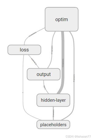
圖 4-35. 可視化全連接網絡的計算圖.
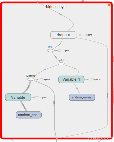
圖 4-36. 可視化全連接網絡的擴展計算圖.
你可以看到可訓練參數和dropout操作在這里是如何呈現的。下面是損失曲線 (Figure 4-37).
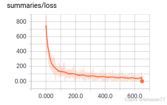
圖4-37. 可視化全連接網絡的損失曲線.
我們放大看仔細點 (Figure 4-38).
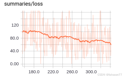
圖 4-38. 局部放大損失曲線
看起來并不平! 這就是使用 minibatch訓練的代價。我們不再有漂亮平滑的損失曲線。


)
)


)
