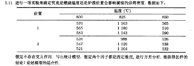
本文是實驗設計與分析（第6版，Montgomery著，傅玨生譯) 第5章析因設計引導5.7節思考題5.11 R語言解題。主要涉及方差分析，正態假設檢驗，殘差分析，交互作用圖。

dataframe<-data.frame(

density=c(570,565,583,528,547,521,1063,1080,1043,988,1026,1004,565,510,590,526,538,532),

Temperature=gl(3,6,18),

position=gl(2,3,18))

summary (dataframe)

dataframe.aov2 <- aov(density~position+Temperature,data=dataframe)

summary (dataframe.aov2)

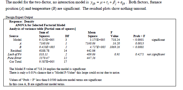
> summary (dataframe.aov2)

??????????? Df Sum Sq Mean Sq F value?? Pr(>F)???

position???? 1?? 7160??? 7160??? 16.2? 0.00125 **

Temperature? 2 945342? 472671? 1069.3 4.92e-16 ***

Residuals?? 14?? 6189???? 442????????????????????

---

Signif. codes:? 0 ‘***’ 0.001 ‘**’ 0.01 ‘*’ 0.05 ‘.’ 0.1 ‘ ’ 1

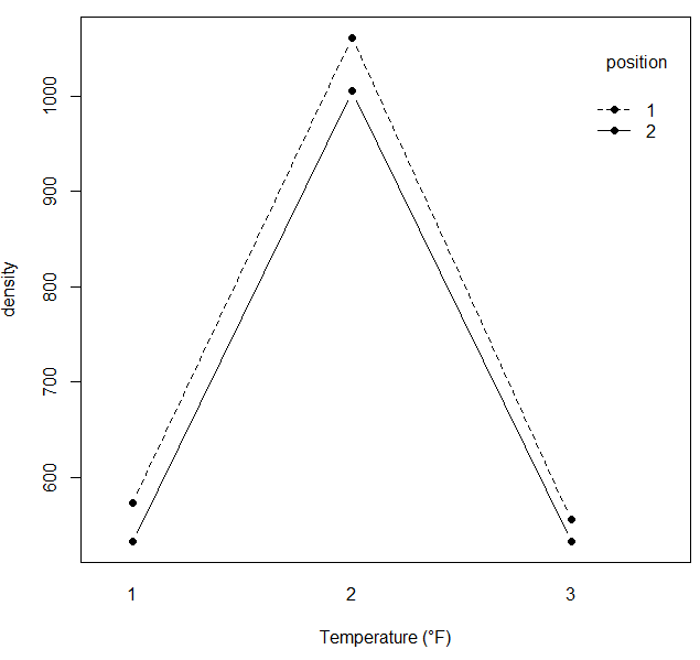
with(dataframe,interaction.plot(Temperature,position,density,type="b",pch=19,fixed=T,xlab="Temperature (°F)",ylab="density"))

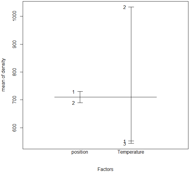
plot.design(density~position*Temperature,data=dataframe)

fit <-lm(density~position+Temperature,data=dataframe)

anova(fit)

> anova(fit)

Analysis of Variance Table

Response: density

??????????? Df Sum Sq Mean Sq? F value??? Pr(>F)???

position???? 1?? 7160??? 7160?? 16.197? 0.001254 **

Temperature? 2 945342? 472671 1069.257 4.924e-16 ***

Residuals?? 14?? 6189???? 442??????????????????????

---

Signif. codes:? 0 ‘***’ 0.001 ‘**’ 0.01 ‘*’ 0.05 ‘.’ 0.1 ‘ ’ 1

summary(fit)

> summary(fit)

Call:

lm(formula = density ~ position + Temperature, data = dataframe)

Residuals:

??? Min????? 1Q? Median????? 3Q???? Max

-53.444? -9.361?? 2.000? 11.639? 26.556

Coefficients:

???????????? Estimate Std. Error t value Pr(>|t|)???

(Intercept)?? 572.278????? 9.911? 57.740? < 2e-16 ***

position2???? -39.889????? 9.911? -4.025? 0.00125 **

Temperature2? 481.667???? 12.139? 39.680 8.69e-16 ***

Temperature3?? -8.833???? 12.139? -0.728? 0.47880???

---

Signif. codes:? 0 ‘***’ 0.001 ‘**’ 0.01 ‘*’ 0.05 ‘.’ 0.1 ‘ ’ 1

Residual standard error: 21.03 on 14 degrees of freedom

Multiple R-squared:? 0.9935,??? Adjusted R-squared:? 0.9922

F-statistic: 718.2 on 3 and 14 DF,? p-value: 1.464e-15

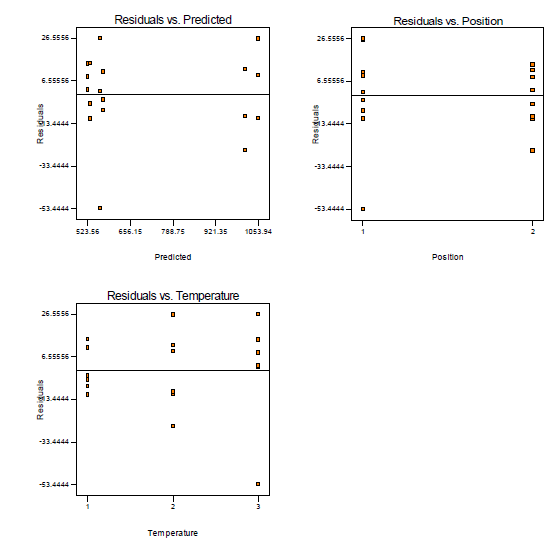
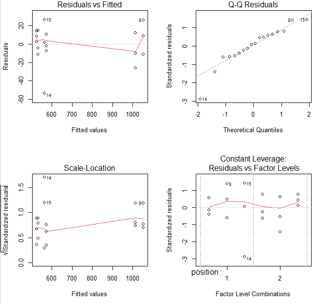
par(mfrow=c(2,2))

plot(fit)

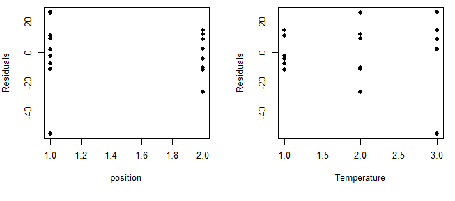
par(mfrow=c(2,2))

plot(as.numeric(dataframe$position), fit$residuals, xlab="position", ylab="Residuals", type="p", pch=16)

plot(as.numeric(dataframe$Temperature), fit$residuals, xlab="Temperature", ylab="Residuals", pch=16)