執行下面這段代碼后,為什么返回的是 2 ?
vector = torch.tensor([7, 7])
vector.shape
為什么返回的是 torch.Size([2])?
當你創建一個PyTorch張量時,它會記住張量中元素的數量和每個維度的大小。在你的代碼中,torch.tensor([7, 7])創建了一個一維張量,其中包含兩個元素:7和7。因為這是一個一維張量,所以.shape屬性返回一個只有一個元素的元組,該元素表示張量的長度。在這種情況下,張量的長度為2,因此返回的形狀是torch.Size([2])。
tensor 的維度
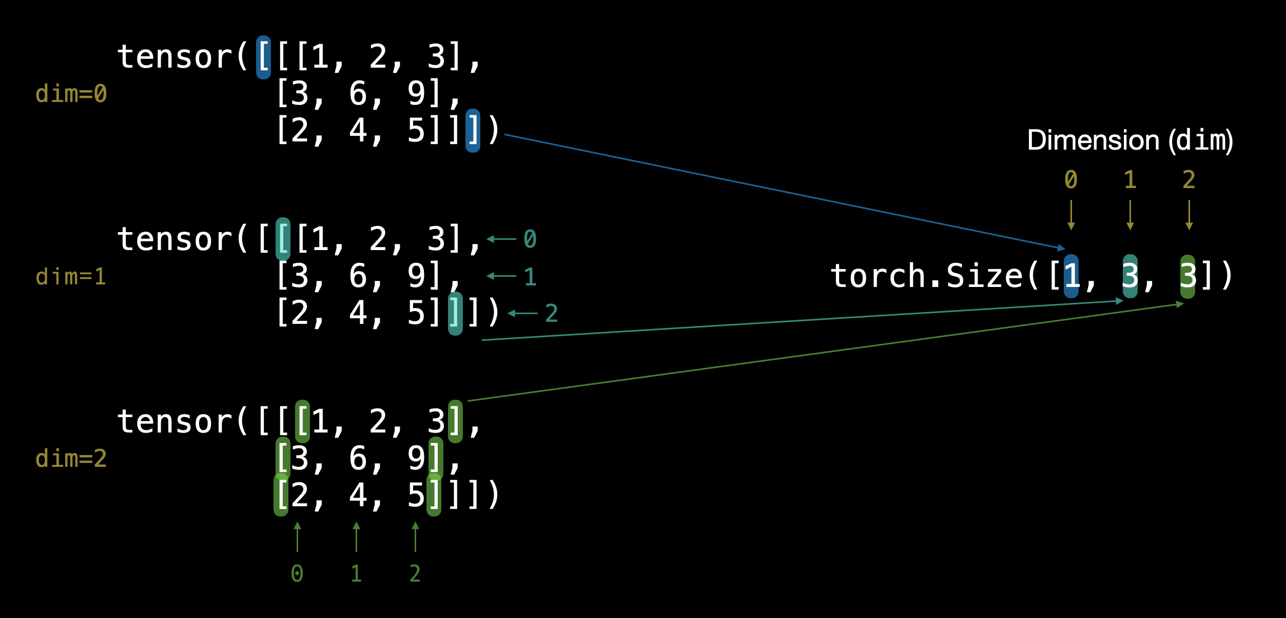
TENSOR = torch.tensor([[[1, 2, 3],[3, 6, 9],[2, 4, 5]]])
TENSOR.ndim
返回的是 [1,3,3] , 如何判斷?有三層 [ ] 括號,將每個 [ ] 括號視為列表,從最里層起,當前列表有幾個并列的元素,TENSOR.ndim 返回的列表最右邊的元素就是幾,然后去掉最外面一層的 [ ] 括號,繼續判斷當前列表有幾個并列的元素,TENSOR.ndim 返回的列表次右邊的元素就是幾,依次類推。
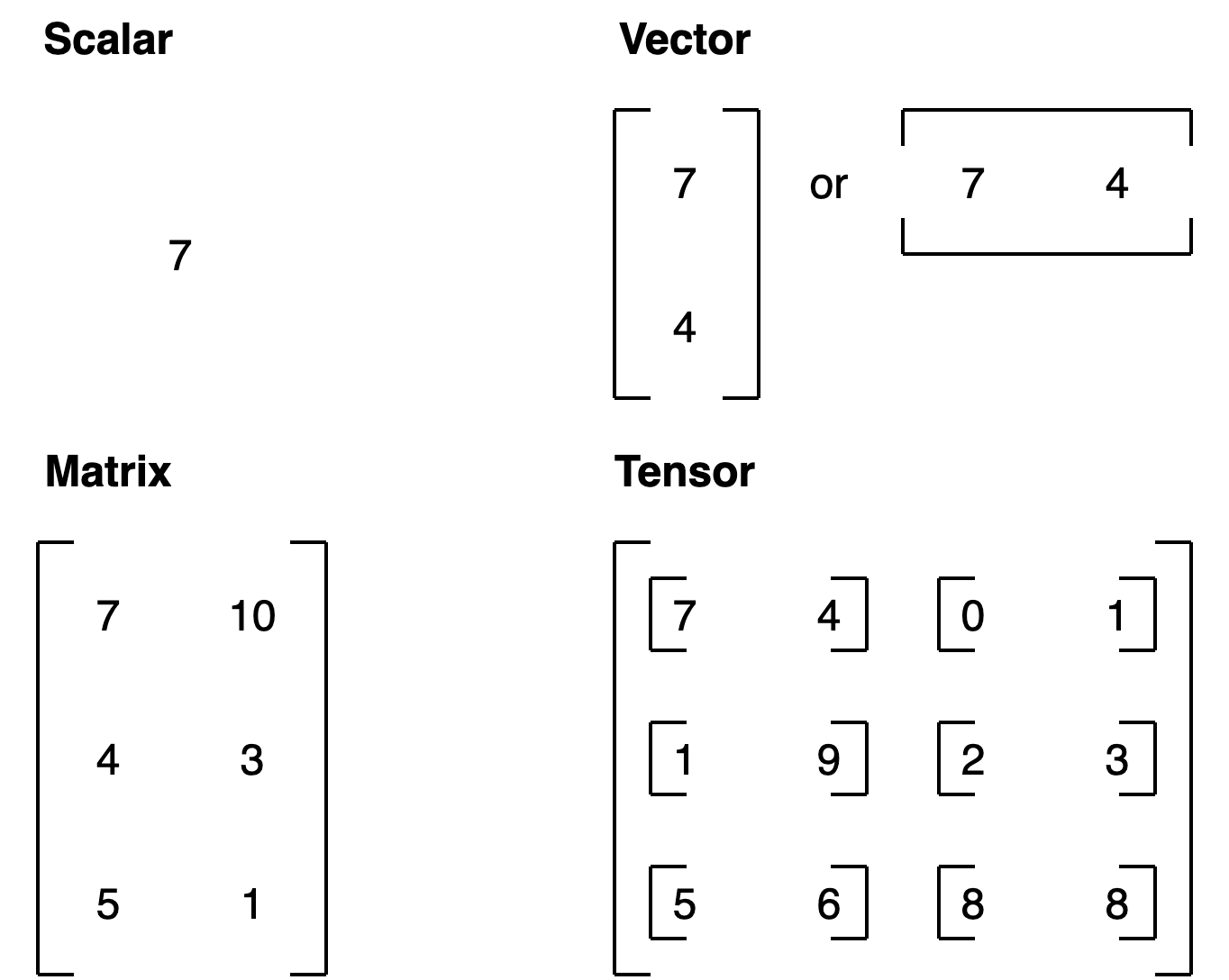
Scalar,Vector,Matrix,Tensor
torch.arange()
torch.arange() 返回的是 PyTorch 中的 tensor,而不是 NumPy 數組。
torch中對tensor的各種切片操作
好的,讓我們使用一個三維張量來詳細解釋各種復雜的切片操作。我們首先創建一個形狀為 2 × 3 × 4 2 \times 3 \times 4 2×3×4 的三維張量:
import torch# 創建一個形狀為 2x3x4 的三維張量
tensor = torch.arange(24).reshape(2, 3, 4)
print("Original Tensor:")
print(tensor)
假設我們有一個如下所示的三維張量:
tensor([[[ 0, 1, 2, 3],[ 4, 5, 6, 7],[ 8, 9, 10, 11]],[[12, 13, 14, 15],[16, 17, 18, 19],[20, 21, 22, 23]]])
1. 選擇特定的切片
選擇第一個維度的第一個子張量
slice_1 = tensor[0, :, :]
print("Slice along the first dimension (index 0):")
print(slice_1)
輸出:
tensor([[ 0, 1, 2, 3],[ 4, 5, 6, 7],[ 8, 9, 10, 11]])
選擇第二個維度的第二個子張量
slice_2 = tensor[:, 1, :]
print("Slice along the second dimension (index 1):")
print(slice_2)
輸出:
tensor([[ 4, 5, 6, 7],[16, 17, 18, 19]])
選擇第三個維度的第三個子張量
slice_3 = tensor[:, :, 2]
print("Slice along the third dimension (index 2):")
print(slice_3)
輸出:
tensor([[ 2, 6, 10],[14, 18, 22]])
2. 高級切片操作
選擇第一個維度的第一個子張量中的第1到第2行(不包括第2行)
slice_4 = tensor[0, 0:1, :]
print("Slice along the first dimension (index 0) and rows 0 to 1:")
print(slice_4)
輸出:
tensor([[0, 1, 2, 3]])
選擇第二個維度的第0和第2行,并選擇所有列
slice_5 = tensor[:, [0, 2], :]
print("Select rows 0 and 2 from the second dimension:")
print(slice_5)
輸出:
tensor([[[ 0, 1, 2, 3],[ 8, 9, 10, 11]],[[12, 13, 14, 15],[20, 21, 22, 23]]])
選擇第三個維度的第1和第3列
slice_6 = tensor[:, :, [1, 3]]
print("Select columns 1 and 3 from the third dimension:")
print(slice_6)
輸出:
tensor([[[ 1, 3],[ 5, 7],[ 9, 11]],[[13, 15],[17, 19],[21, 23]]])
3. 使用布爾張量進行索引
選擇大于10的元素
mask = tensor > 10
slice_7 = tensor[mask]
print("Elements greater than 10:")
print(slice_7)
輸出:
tensor([11, 12, 13, 14, 15, 16, 17, 18, 19, 20, 21, 22, 23])
4. 使用長整型張量進行索引
選擇第1和第3列的數據
indices = torch.tensor([1, 3])
slice_8 = tensor[:, :, indices]
print("Select columns indexed by [1, 3]:")
print(slice_8)
輸出:
tensor([[[ 1, 3],[ 5, 7],[ 9, 11]],[[13, 15],[17, 19],[21, 23]]])
5. 花式索引
使用多個索引數組
rows = torch.tensor([0, 1])
cols = torch.tensor([2, 3])
slice_9 = tensor[0, rows, cols]
print("Fancy indexing with rows and cols:")
print(slice_9)
輸出:
tensor([2, 7])
通過這些示例,希望你對 PyTorch 中的張量索引和切片操作有了更深入的理解。這些操作在數據預處理、特征提取和神經網絡模型的實現中非常重要。
torch 中 tensor 的各種乘法
在 PyTorch 中,有多種實現張量相乘的方式,每種方式在實現上有一些差異,有些是就地操作,有些不是。以下是幾種主要的實現方式:
1. 元素級相乘 (Element-wise Multiplication)
要求兩個 tensor 的 shape 一致
使用 * 操作符
import torcha = torch.tensor([[1, 2], [3, 4]])
b = torch.tensor([[5, 6], [7, 8]])result = a * b
print(result)
使用 torch.mul()
result = torch.mul(a, b)
print(result)
就地操作
使用 mul_() 方法:
a.mul_(b)
print(a)
2. 矩陣乘法 (Matrix Multiplication)
使用 @ 操作符 (Python 3.5+)
result = a @ b.T  # 轉置 b 以使其形狀匹配矩陣乘法要求
print(result)
使用 torch.matmul()
result = torch.matmul(a, b.T)
print(result)
使用 torch.mm()(僅適用于二維張量)
result = torch.mm(a, b.T)
print(result)
3. 廣義點積 (Dot Product for 1D tensors)
使用 torch.dot()
c = torch.tensor([1, 2, 3])
d = torch.tensor([4, 5, 6])result = torch.dot(c, d)
print(result)
4. 批量矩陣乘法 (Batch Matrix Multiplication)
使用 torch.bmm()
e = torch.randn(10, 3, 4)  # 形狀為 (batch_size, m, n)
f = torch.randn(10, 4, 5)  # 形狀為 (batch_size, n, p)result = torch.bmm(e, f)
print(result)
5. 廣播相乘 (Broadcast Multiplication)
張量會自動廣播到兼容的形狀。
g = torch.tensor([1, 2, 3])
h = torch.tensor([[1], [2], [3]])result = g * h
print(result)
就地操作總結
就地操作會直接修改原始張量的值,通常以 _ 結尾:
a.mul_(b):就地進行元素級相乘
非就地操作會創建新的張量并返回結果,而不改變輸入張量的值。
這些不同的乘法操作方式在不同的應用場景中有不同的用途,根據需要選擇適合的乘法方式。


)


)
)

【如何在Qt Creator中創建新工程】)