VGG論文解析—Very Deep Convolutional Networks for Large-Scale Image Recognition -2015

研究背景

大規模圖像識別的深度卷積神經網絡 VGG（牛津大學視覺幾何組）

認識數據集：ImageNet的大規模圖像識別挑戰賽

LSVRC-2014：ImageNet Large Scale Visual Recoanition Challenge(14年的相關比賽)

相關研究借鑒：

AlexNet ZFNet OverFeat

研究成果

• ILSVRC定位冠軍，分類亞軍

• 開源VGG16，VGG19

• 開啟小卷積核，深度卷積模型時代3*3卷積核成為主流模型

LSVRC: ImageNet Large Scale Visual Recognition Challenge 是李飛飛等人于2010年創辦的圖像識別挑戰賽，自2010起連續舉辦8年，極大地推動計算機視覺發展。

比賽項目涵蓋：圖像分類（Classification）、目標定位（Object localization）、目標檢測（Object detection）、視頻目標檢測（Object detection from video)、場景分類(Scene classification)、場景解析(Scene parsing)

競賽中脫穎而出大量經典模型：
alexnet，vgg，googlenet ，resnet，densenet等

1. AlexNet：ILSVRC-2012分類冠軍，里程碑的CNN模型
2. ZFNet：ILSVRC-2013分類冠軍方法，對AlexNet改進
3. OverFeat：ILSVRC-2013定位冠軍，集分類、定位和檢測于一體的卷積網絡方法(即將全連接層替換為1x1的卷積層)

論文精讀

摘要

In this work we investigate the effect of the convolutional network depth on its accuracy in the large-scale image recognition setting. Our main contribution is a thorough evaluation of networks of increasing depth using an architecture with very small (3×3) convolution filters, which shows that a significant improvement on the prior-art configurations can be achieved by pushing the depth to 16–19 weight layers. These findings were the basis of our ImageNet Challenge 2014 submission, where our team secured the first and the second places in the localisation and classification tracks respectively. We also show that our representations
generalise well to other datasets, where they achieve state-of-the-art results. We have made our two best-performing ConvNet models publicly available to facilitate further research on the use of deep visual representations in computer vision.

摘要進行解讀

1. 本文主題：在大規模圖像識別任務中，探究卷積網絡深度對分類準確率的影響
2. 主要工作：研究3*3卷積核增加網絡模型深度的卷積網絡的識別性能，同時將模型加深到16-19層
3. 本文成績：VGG在ILSVRC-2014獲得了定位任務冠軍和分類任務亞軍
4. 泛化能力：VGG不僅在ILSVRC獲得好成績，在別的數據集中表現依舊優異
5. 開源貢獻：開源兩個最優模型，以加速計算機視覺中深度特征表示的進一步研究

快速泛讀論文確定小標題的結構

1. Introduction
2. ConvNet Configurations

• 2.1 Architecture
• 2.2 Configuratoins
• 2.3 Discussion

3. Classification Framework

• 3.1 Training
• 3.2Testing
• 3.3ImplementationDetails

4. Classification Experiments

• 4.1 Singlescaleevaluation
• 4.2 Multi-Scale evaluation
• 4.3 Multi-Cropevaluation
• 4.4 ConvNetFusion
• 4.5 Comparison with the state of the art

5. Conclusion

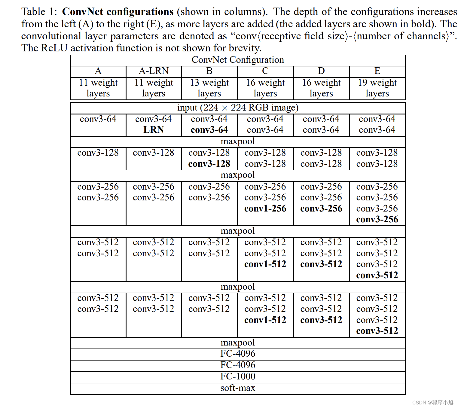
根據圖表結構：論文中提出了A A-LRN B C D E等五種VGG網絡對應的論文結構。

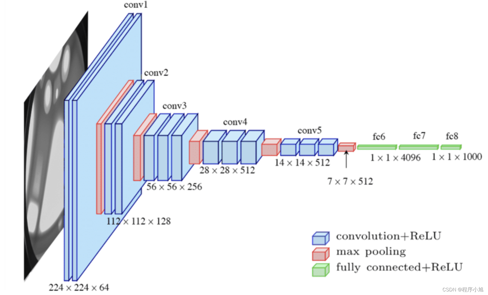
VGG網絡結構

模型結構

During training, the input to our ConvNets is a fixed-size 224 × 224 RGB image. The only preprocessing we do is subtracting the mean RGB value, computed on the training set, from each pixel.
The image is passed through a stack of convolutional (conv.) layers, where we use filters with a very small receptive field: 3 × 3 (which is the smallest size to capture the notion of left/right, up/down,center). In one of the configurations we also utilise 1 × 1 convolution filters, which can be seen as a linear transformation of the input channels (followed by non-linearity). The convolution stride is fixed to 1 pixel; the spatial padding of conv. layer input is such that the spatial resolution is preserved after convolution, i.e. the padding is 1 pixel for 3 × 3 conv. layers. Spatial pooling is carried out by five max-pooling layers, which follow some of the conv. layers (not all the conv. layers are followed by max-pooling). Max-pooling is performed over a 2 × 2 pixel window, with stride 2.
A stack of convolutional layers (which has a different depth in different architectures) is followed by three Fully-Connected (FC) layers: the first two have 4096 channels each, the third performs 1000- way ILSVRC classification and thus contains 1000 channels (one for each class). The final layer is the soft-max layer. The configuration of the fully connected layers is the same in all networks. All hidden layers are equipped with the rectification (ReLU (Krizhevsky et al., 2012)) non-linearity. We note that none of our networks (except for one) contain Local Response Normalisation (LRN) normalisation (Krizhevsky et al., 2012): as will be shown in Sect. 4, such normalisation does not improve the performance on the ILSVRC dataset, but leads to increased memory consumption and computation time. Where applicable, the parameters for the LRN layer are those of (Krizhevsky et al., 2012).

論文的原文中提到了整個VGG網絡的輸入是224 x 224的RGB三通道的彩色圖片。使用了大小為3x3的卷積核（也嘗試的使用了1x1的卷積核）同時使用了2x2的最大池化，步長為2同時不在使用LRN這種方法

11 weight layers in the network A(8 conv. and 3 FC layers) to 19 weight layers in the network E (16 conv. and 3 FC layers).

VGG11由8個卷積層和3個全連接層組成，VGG19由16個卷積層和3個全連接層組成

整個全連接層與AlexNet相同都是4096 x 4096 x1000，最后通過softmax函數完成1000分類、

整個VGG全部采用3x3的卷積

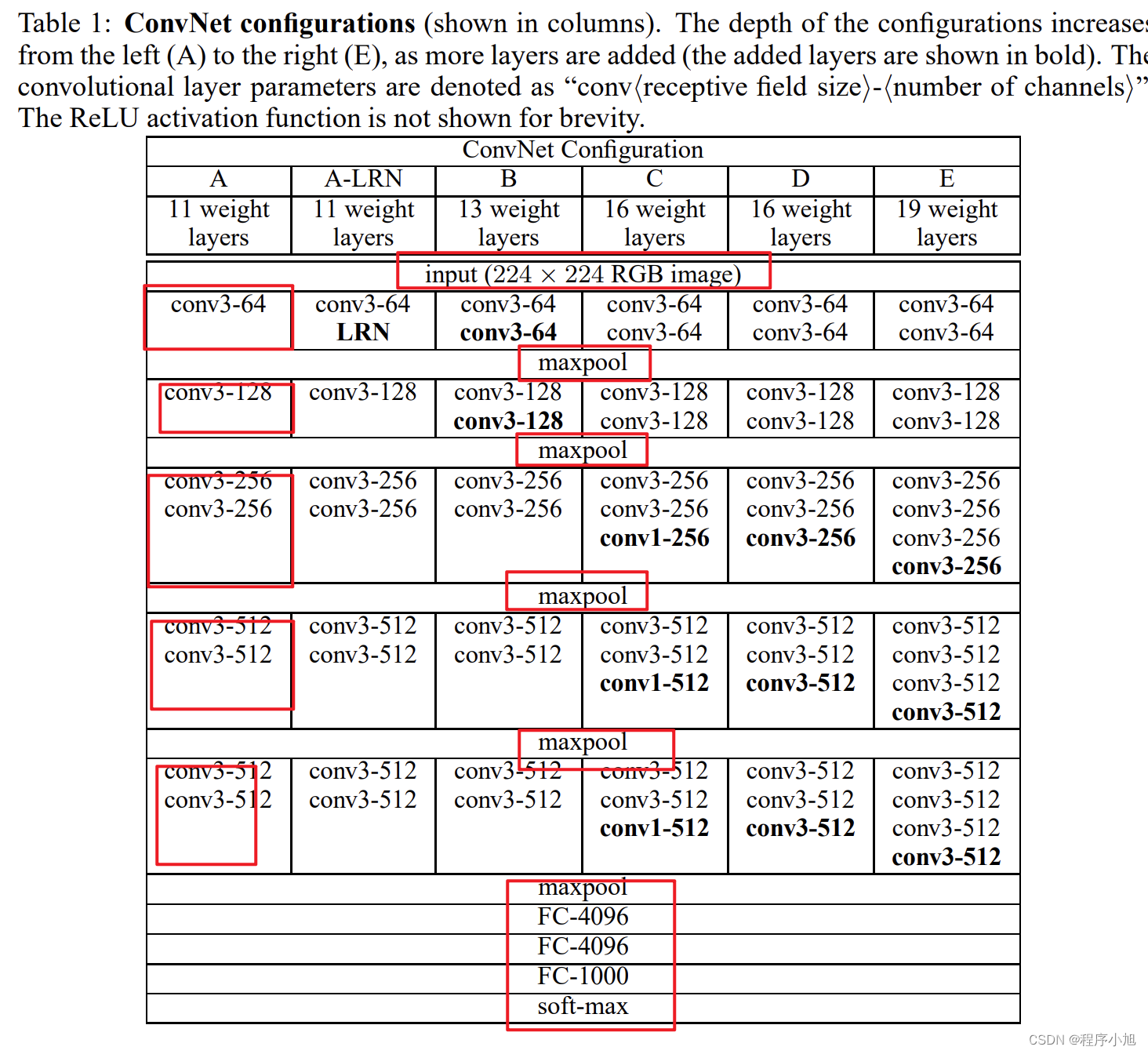
對A（VGG11）的過程和共性進行解讀

首先論文中使用的是：224x224x3的一個輸入，我們設置的是3x3的卷積核，論文中的作者進行了padding填充（1）保持經過卷積之后的圖片大小不變。（conv-64）因此經過了第一層的卷積之后，得到了224x224x64的輸出。

而最大池化的步驟2x2且步長為2
$$F_o=?\frac{F_{\text{in?}}?k+2p}{s}?+1$$

按照公式進行計算：
（224-2）/2 +1=112 因此輸出是112x112的大小，在512之前，每次的通道數翻倍。

卷積不改變圖片的大小，池化使得圖片的大小減半，通道數翻倍

共性

1. 5個maxpool
2. maxpool后，特征圖通道數翻倍直至512
3. 3個FC層進行分類輸出
4. maxpool之間采用多個卷積層堆疊，對特征進行提取和抽象

參數計算

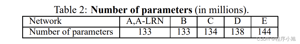
說明了網絡的層數變化，對參數的變化影響不大

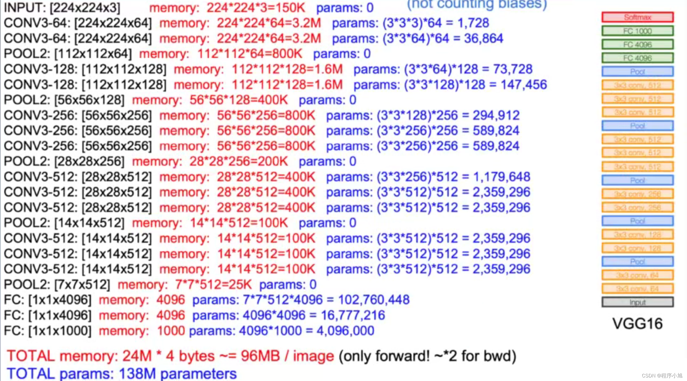
$$F_i\times \left(K_{\mathrm{s}}\times K_{\mathrm{s}}\right)\times K_n+K_n$$

模型演變

A：11層卷積(VGG11)
A-LRN：基于A增加一個LRN
B：第1，2個block中增加1個卷積33卷積
C：第3，4，5個block分別增加1個11卷積
表明增加非線性有益于指標提升
D：第3，4，5個block的11卷積替換為33(VGG16)
E：第3，4，5個block再分別增加1個3*3卷積

其中最為常用的結構就是A中的VGG11和D中的VGG16

VGG的特點

1. 堆疊3x3的卷積核

增大感受野2個33堆疊等價于1個553個33堆疊等價于1個77

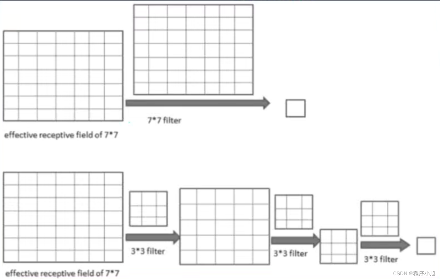
增加非線性激活函數，增加特征抽象能力
減少訓練參數
可看成7 * 7卷積核的正則化，強迫7 * 7分解為3 * 3

假設輸入，輸出通道均為C個通道
一個77卷積核所需參數量：7 * 7 C * C=49C2
三個33卷積核所需參數量：3（3 * 3* C *C）=27C2
參數減少比：（49-27）/49~44%

之后的數據處理過程和測試過程的相關的內容，放到之后在進行下一次的解讀，通過這一次主要要理解的是VGG的網絡結構