一句話總結：

這篇論文通過讓合成數據”教“學生網絡沿著專家軌跡走，從而在極小數據量下實現高性能，開創了數據集蒸餾的新范式。后面很多工作都基于這篇工作來進行改進

---

CVPR2022 github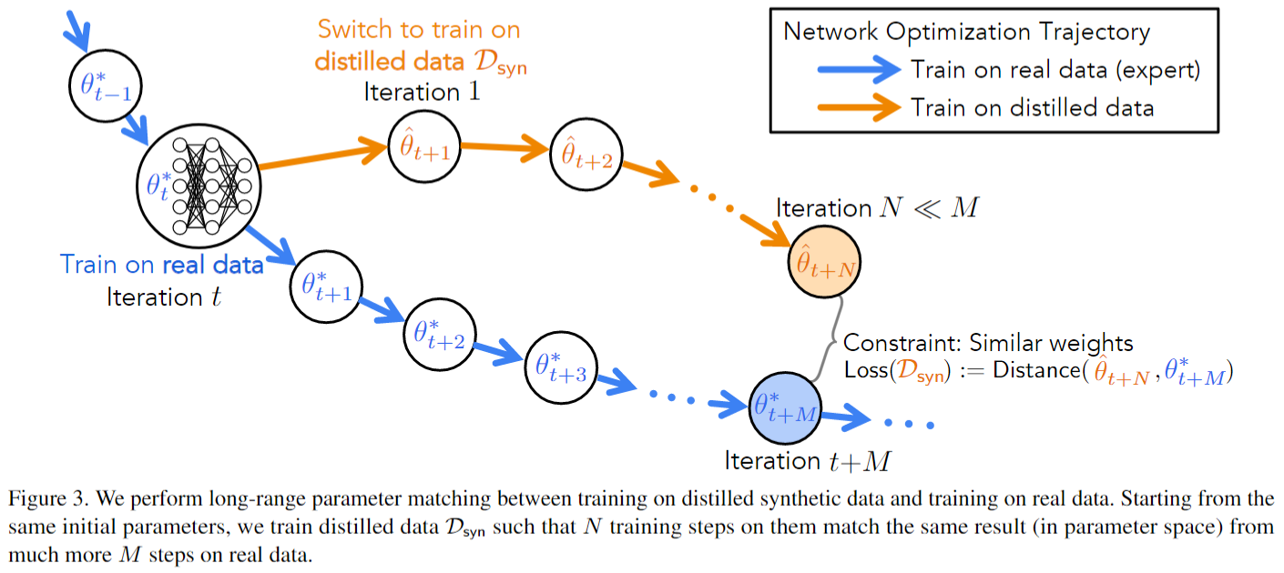

1.動機與背景

• 數據集蒸餾（Dataset Distillation）：用一個極小的合成數據集$D_{syn}$訓練模型，使其在真實測試集上的性能接近用完整訓練集$D_{real}$訓練的模型。
• 局限性：先前的梯度匹配方法（詳細可看另外一篇博客）只對齊”每一步的梯度“，忽視了模型訓練的長程動態；而完全展開多步優化又代價太高、易不穩定。

---

2.核心方法：軌跡匹配（Trajectory Matching）

1. 專家軌跡（Expert Trajectories）

   • 離線預先訓練若干網絡，每隔一個epoch保存一次模型參數{θt?}t=0T\{\theta_{t}^{*} \}_{t=0}^{T}{θt??}t=0T?, 得到”專家軌跡“。
   • 這些軌跡代表真實數據訓練的”理想路徑“，可重復復用，避免再蒸餾時重新訓練大模型。

2. 軌跡對齊（Long-Range Match）

   • 在合成數據上，從專家軌跡的某個起點 ${\theta }_t^{?}$ 初始化”學生“參數 $\widehat{{\theta }_t}$
   • 在$D_{syn}$上做N步梯度下降：

   ? ${\hat{\theta }}_{t+n+1}={\hat{\theta }}_{t+n}?\alpha {?}_{\theta }?(D_{syn};{\hat{\theta }}_{t+n})$

   • 對齊學生在步t+N的參數${\hat{\theta }}_{t+N}$與專家在更遠的參數${\theta }_{t+M}^{?}$, 損失為：
     $$\mathcal{L}=\frac{{\Vert {\hat{\theta }}_{t+N}?{\theta }_{t+M}^{?}\Vert }_2^2}{{\Vert {\theta }_t^{?}?{\theta }_{t+M}^{?}\Vert }_2^2}$$
     分母做歸一化，放大信號并自動平衡各層尺度。

   • 外循環（更新合成數據）+內循環（在$D_{syn}$上模擬N步）結果，借助create_graph=True保留計算圖，將對齊損失反向傳播到合成圖像及可學的學生學習率$\alpha$。

3. 內存優化

   • 不一次性對合成集做匹配，而是在學生網絡的內循環中按小批次（跨類別但每類少量）更新，既保證”每張圖像都被看過“，又大幅節省顯存。

---

3.實驗與效果

• 小樣本極端場景：CIFAR-10/100、SVHN 上每類僅 1 或 10 張合成樣本，軌跡匹配比梯度匹配提升約 5–10%。
• 多分辨率驗證：Tiny-ImageNet (64×64)、ImageNette/ImageWoof (128×128) 均取得顯著增益。
• 跨架構泛化：雖針對某一網絡訓練，合成集在 ResNet-18、VGG、AlexNet 等不同模型上依舊表現穩健。
• 消融分析：軌跡長度 MM、內循環步數 NN、匹配目標（參數 vs 輸出）、專家軌跡數量等均對性能有明顯影響，驗證設計合理性。

---

4.個人思考與啟發

• ”長程軌跡對齊“勝于”短程梯度對齊“：對齊訓練軌跡（”路徑“）往往比對齊某一步”梯度“更能保證學習行為一致。
• 雖然可以通過預存儲軌跡和小批次策略提高效率，但是仍然很耗內存。在訓練教師模型的時候，需要把多個教師軌跡存儲下來，在訓練學生模型的時候需要把訓練的參數記錄下來，占用大量的內存與顯存。同時復雜的雙層優化，難以避免復雜度高。

---

主體代碼

   ''' training '''# 將合成圖像與LR設為可優化image_syn = image_syn.detach().to(args.device).requires_grad_(True)syn_lr = syn_lr.detach().to(args.device).requires_grad_(True)optimizer_img = torch.optim.SGD([image_syn], lr=args.lr_img, momentum=0.5)# 學習率也設置為可優化optimizer_lr = torch.optim.SGD([syn_lr], lr=args.lr_lr, momentum=0.5)optimizer_img.zero_grad()criterion = nn.CrossEntropyLoss().to(args.device)print('%s training begins'%get_time())# 專家軌跡路徑expert_dir = os.path.join(args.buffer_path, args.dataset)if args.dataset == "ImageNet":expert_dir = os.path.join(expert_dir, args.subset, str(args.res))if args.dataset in ["CIFAR10", "CIFAR100"] and not args.zca:expert_dir += "_NO_ZCA"expert_dir = os.path.join(expert_dir, args.model)print("Expert Dir: {}".format(expert_dir))# 加載或部分加載專家軌跡if args.load_all:buffer = []n = 0while os.path.exists(os.path.join(expert_dir, "replay_buffer_{}.pt".format(n))):buffer = buffer + torch.load(os.path.join(expert_dir, "replay_buffer_{}.pt".format(n)))n += 1if n == 0:raise AssertionError("No buffers detected at {}".format(expert_dir))else:expert_files = []n = 0while os.path.exists(os.path.join(expert_dir, "replay_buffer_{}.pt".format(n))):expert_files.append(os.path.join(expert_dir, "replay_buffer_{}.pt".format(n)))n += 1if n == 0:raise AssertionError("No buffers detected at {}".format(expert_dir))file_idx = 0expert_idx = 0random.shuffle(expert_files)if args.max_files is not None:expert_files = expert_files[:args.max_files]print("loading file {}".format(expert_files[file_idx]))buffer = torch.load(expert_files[file_idx])if args.max_experts is not None:buffer = buffer[:args.max_experts]random.shuffle(buffer)# 記錄最佳精度與方差best_acc = {m: 0 for m in model_eval_pool}best_std = {m: 0 for m in model_eval_pool}# --- 蒸餾迭代主循環 ---for it in range(0, args.Iteration+1):save_this_it = False   # 標記本次迭代是否是要保存的最佳合成數據# 將當前迭代進度記錄到 Weights & Biases (W&B)# writer.add_scalar('Progress', it, it)wandb.log({"Progress": it}, step=it)''' Evaluate synthetic data '''# 如果當前迭代在預設的評估點列表中，則評估合成數據在隨機模型上的表現if it in eval_it_pool:for model_eval in model_eval_pool:print('-------------------------\nEvaluation\nmodel_train = %s, model_eval = %s, iteration = %d'%(args.model, model_eval, it))# 打印使用的數據增強策略if args.dsa:print('DSA augmentation strategy: \n', args.dsa_strategy)print('DSA augmentation parameters: \n', args.dsa_param.__dict__)else:print('DC augmentation parameters: \n', args.dc_aug_param)accs_test = []  # 存儲每次評估的測試準確率accs_train = []  # 存儲每次評估的訓練準確率# 重復num_eval 次隨機初始化的模型評估，以平均化隨機性for it_eval in range(args.num_eval):# 隨機初始化一個新模型net_eval = get_network(model_eval, channel, num_classes, im_size).to(args.device) # get a random modeleval_labs = label_syn# 固定合成圖像與標簽，避免在評估時被意外修改with torch.no_grad():image_save = image_synimage_syn_eval, label_syn_eval = copy.deepcopy(image_save.detach()), copy.deepcopy(eval_labs.detach()) # avoid any unaware modification# 將當前合成學習率傳遞給評估函數args.lr_net = syn_lr.item()# 用合成數據訓練并評估 net_eval，返回 (loss, train_acc, test_acc)_, acc_train, acc_test = evaluate_synset(it_eval, net_eval, image_syn_eval, label_syn_eval, testloader, args, texture=args.texture)accs_test.append(acc_test)accs_train.append(acc_train)accs_test = np.array(accs_test)accs_train = np.array(accs_train)acc_test_mean = np.mean(accs_test)acc_test_std = np.std(accs_test)# 如果有新的最佳平均準確率，則更新best_acc并標記保存if acc_test_mean > best_acc[model_eval]:best_acc[model_eval] = acc_test_meanbest_std[model_eval] = acc_test_stdsave_this_it = Trueprint('Evaluate %d random %s, mean = %.4f std = %.4f\n-------------------------'%(len(accs_test), model_eval, acc_test_mean, acc_test_std))# 將評估結果記錄到 W&Bwandb.log({'Accuracy/{}'.format(model_eval): acc_test_mean}, step=it)wandb.log({'Max_Accuracy/{}'.format(model_eval): best_acc[model_eval]}, step=it)wandb.log({'Std/{}'.format(model_eval): acc_test_std}, step=it)wandb.log({'Max_Std/{}'.format(model_eval): best_std[model_eval]}, step=it)# 如果評估改進或周期點，保存合成圖像到 W&B 與本地if it in eval_it_pool and (save_this_it or it % 1000 == 0):with torch.no_grad():image_save = image_syn.cuda()save_dir = os.path.join(".", "logged_files", args.dataset, wandb.run.name)if not os.path.exists(save_dir):os.makedirs(save_dir)# 保存當前迭代的合成圖像與標簽torch.save(image_save.cpu(), os.path.join(save_dir, "images_{}.pt".format(it)))torch.save(label_syn.cpu(), os.path.join(save_dir, "labels_{}.pt".format(it)))# 如果達成新最佳，還額外保存為 bestif save_this_it:torch.save(image_save.cpu(), os.path.join(save_dir, "images_best.pt".format(it)))torch.save(label_syn.cpu(), os.path.join(save_dir, "labels_best.pt".format(it)))# 將像素分布記錄為 W&B 直方圖wandb.log({"Pixels": wandb.Histogram(torch.nan_to_num(image_syn.detach().cpu()))}, step=it)# 可視化合成圖像：若 ipc<50 或 強制保存，則進行網格化展示if args.ipc < 50 or args.force_save:upsampled = image_saveif args.dataset != "ImageNet":# 針對 CIFAR 類數據，將低分辨率圖像放大 4 倍以便觀察upsampled = torch.repeat_interleave(upsampled, repeats=4, dim=2)upsampled = torch.repeat_interleave(upsampled, repeats=4, dim=3)grid = torchvision.utils.make_grid(upsampled, nrow=10, normalize=True, scale_each=True)wandb.log({"Synthetic_Images": wandb.Image(torch.nan_to_num(grid.detach().cpu()))}, step=it)wandb.log({'Synthetic_Pixels': wandb.Histogram(torch.nan_to_num(image_save.detach().cpu()))}, step=it)for clip_val in [2.5]:std = torch.std(image_save)mean = torch.mean(image_save)upsampled = torch.clip(image_save, min=mean-clip_val*std, max=mean+clip_val*std)if args.dataset != "ImageNet":upsampled = torch.repeat_interleave(upsampled, repeats=4, dim=2)upsampled = torch.repeat_interleave(upsampled, repeats=4, dim=3)grid = torchvision.utils.make_grid(upsampled, nrow=10, normalize=True, scale_each=True)wandb.log({"Clipped_Synthetic_Images/std_{}".format(clip_val): wandb.Image(torch.nan_to_num(grid.detach().cpu()))}, step=it)# 如果使用 ZCA 預處理，還需要保存和可視化反變換后的圖像if args.zca:image_save = image_save.to(args.device)image_save = args.zca_trans.inverse_transform(image_save)image_save.cpu()torch.save(image_save.cpu(), os.path.join(save_dir, "images_zca_{}.pt".format(it)))upsampled = image_saveif args.dataset != "ImageNet":upsampled = torch.repeat_interleave(upsampled, repeats=4, dim=2)upsampled = torch.repeat_interleave(upsampled, repeats=4, dim=3)grid = torchvision.utils.make_grid(upsampled, nrow=10, normalize=True, scale_each=True)wandb.log({"Reconstructed_Images": wandb.Image(torch.nan_to_num(grid.detach().cpu()))}, step=it)wandb.log({'Reconstructed_Pixels': wandb.Histogram(torch.nan_to_num(image_save.detach().cpu()))}, step=it)for clip_val in [2.5]:std = torch.std(image_save)mean = torch.mean(image_save)upsampled = torch.clip(image_save, min=mean - clip_val * std, max=mean + clip_val * std)if args.dataset != "ImageNet":upsampled = torch.repeat_interleave(upsampled, repeats=4, dim=2)upsampled = torch.repeat_interleave(upsampled, repeats=4, dim=3)grid = torchvision.utils.make_grid(upsampled, nrow=10, normalize=True, scale_each=True)wandb.log({"Clipped_Reconstructed_Images/std_{}".format(clip_val): wandb.Image(torch.nan_to_num(grid.detach().cpu()))}, step=it)# 記錄當前合成學習率到 W&Bwandb.log({"Synthetic_LR": syn_lr.detach().cpu()}, step=it)# --- 學生模型初始化與專家軌跡抽樣 ---# 隨機初始化學生網絡并轉換為 ReparamModule 以支持扁平化權重student_net = get_network(args.model, channel, num_classes, im_size, dist=False).to(args.device)  # get a random modelstudent_net = ReparamModule(student_net)if args.distributed:student_net = torch.nn.DataParallel(student_net)student_net.train()# 計算網絡參數總數，用于后續損失歸一化num_params = sum([np.prod(p.size()) for p in (student_net.parameters())])# 從 buffer 中輪詢或隨機獲取一條專家軌跡if args.load_all:expert_trajectory = buffer[np.random.randint(0, len(buffer))]else:expert_trajectory = buffer[expert_idx]expert_idx += 1if expert_idx == len(buffer):expert_idx = 0file_idx += 1# 如果切換到下一個 buffer 文件，則重新加載并打亂if file_idx == len(expert_files):file_idx = 0random.shuffle(expert_files)print("loading file {}".format(expert_files[file_idx]))if args.max_files != 1:del bufferbuffer = torch.load(expert_files[file_idx])if args.max_experts is not None:buffer = buffer[:args.max_experts]random.shuffle(buffer)# 從專家軌跡中隨機選擇起始epoch和目標epoch參數start_epoch = np.random.randint(0, args.max_start_epoch)starting_params = expert_trajectory[start_epoch]target_params = expert_trajectory[start_epoch+args.expert_epochs]# 將參數列表展平成單個向量target_params = torch.cat([p.data.to(args.device).reshape(-1) for p in target_params], 0)student_params = [torch.cat([p.data.to(args.device).reshape(-1) for p in starting_params], 0).requires_grad_(True)]starting_params = torch.cat([p.data.to(args.device).reshape(-1) for p in starting_params], 0)syn_images = image_syn # 合成圖像集合y_hat = label_syn.to(args.device)# 準備列表保存中間參數損失與距離param_loss_list = []param_dist_list = []indices_chunks = [] # 用于分批操作的索引緩存# --- 合成數據多步梯度更新模擬 ---for step in range(args.syn_steps):# 如果當前無可用indices_chunks，則重新打亂并拆分if not indices_chunks:indices = torch.randperm(len(syn_images))indices_chunks = list(torch.split(indices, args.batch_syn))these_indices = indices_chunks.pop()x = syn_images[these_indices]   # 取當前批次的合成圖像this_y = y_hat[these_indices]   # 對應標簽# texture 模式下，進行隨機平移并裁剪模擬紋理拼接if args.texture:x = torch.cat([torch.stack([torch.roll(im, (torch.randint(im_size[0]*args.canvas_size, (1,)), torch.randint(im_size[1]*args.canvas_size, (1,))), (1,2))[:,:im_size[0],:im_size[1]] for im in x]) for _ in range(args.canvas_samples)])this_y = torch.cat([this_y for _ in range(args.canvas_samples)])# 可微增強替代普通數據增強if args.dsa and (not args.no_aug):x = DiffAugment(x, args.dsa_strategy, param=args.dsa_param)if args.distributed:forward_params = student_params[-1].unsqueeze(0).expand(torch.cuda.device_count(), -1)else:forward_params = student_params[-1]# 前向計算 logitsx = student_net(x, flat_param=forward_params)ce_loss = criterion(x, this_y)# 計算損失對扁平化參數的梯度（保留圖以繼續反向到合成圖像）grad = torch.autograd.grad(ce_loss, student_params[-1], create_graph=True)[0]# 更新學生參數向下一個步長student_params.append(student_params[-1] - syn_lr * grad)# --- 計算參數匹配損失 ---param_loss = torch.tensor(0.0).to(args.device)param_dist = torch.tensor(0.0).to(args.device)param_loss += torch.nn.functional.mse_loss(student_params[-1], target_params, reduction="sum")param_dist += torch.nn.functional.mse_loss(starting_params, target_params, reduction="sum")param_loss_list.append(param_loss)param_dist_list.append(param_dist)# 歸一化：先按參數總數，再除以起點-目標距離param_loss /= num_paramsparam_dist /= num_paramsparam_loss /= param_distgrand_loss = param_loss# --- 更新合成圖像與合成學習率 ---optimizer_img.zero_grad()optimizer_lr.zero_grad()grand_loss.backward()optimizer_img.step()optimizer_lr.step()# 記錄損失與起始 epochwandb.log({"Grand_Loss": grand_loss.detach().cpu(),"Start_Epoch": start_epoch})# 清理中間梯度緩存，避免顯存泄漏for _ in student_params:del _# 每 10 次迭代打印一次損失信息if it%10 == 0:print('%s iter = %04d, loss = %.4f' % (get_time(), it, grand_loss.item()))wandb.finish()

算法邏輯總結

1. 準備”專家示范“
   • 先用真實大數據集訓練一個（或多組）模型，把模型再每個訓練輪/每步的所有參數都記下來，這條參數隨實踐變化的記錄叫做”專家軌跡“。
2. 初始化”學生“
   • 選軌跡上某個時間點，把學生網絡的參數初始化為老師當時的狀態。這樣學生和老師從同一個起點出發。
3. 學生用合成數據學N步
   • 用我們的小合成數據集讓學生網絡做N步梯度下降（就是跑N個小批次的訓練）。
   • 記錄學生跑完這N步后得到的新參數。
4. 對齊”未來“
   • 看老師在真實訓練中，從同一個起點走M步后參數是怎么樣，把學生此刻的參數和老師未來第M步的參數做對比。
   • 差距越小，說明學生越像老師；差距越大，說明合成數據還不夠好。
5. 更新合成數據
   • 把這個”未來對齊“誤差當作損失，反向傳播回去，去調整我們的小合成圖像（和一個”學生學習率“參數）。
   • 目的就是讓下一輪學生訓練時候，能更快更準確地朝著老師的軌跡走。
6. 重復很多輪
   • 每輪都重新從專家軌跡選一個起點，反復做上面四步，讓小合成數據不斷進化、越來越”聰明“。