• 🍨 本文為🔗365天深度學習訓練營 中的學習記錄博客
• 🍖 原作者：K同學啊 | 接輔導、項目定制

一、 前期準備

語言環境：Python3.7.8
編譯器選擇：VSCode
深度學習環境：TensorFlow
數據集：本地數據集

1.1 設置GPU

本文使用CPU環境

'''
LSTM-實現火災預測
'''import tensorflow as tfgpus = tf.config.list_physical_devices("GPU")if gpus:gpu0 = gpus[0]tf.config.experimental.set_memory_growth(gpu0,true)tf.config.set_visible_devices([gpu0],"GPU")print("GPU: ",gpus)
else:print("CPU:")

輸出：

1.2 導入數據

下載數據集文件woodpine2.csv到本地，使用絕對路徑進行訪問：

# 2.1 導入數據
import  pandas as pd
import numpy as np
import matplotlib.pyplot as plt
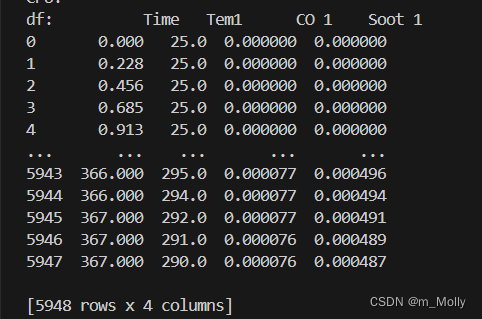
import seaborn as snsdf = pd.read_csv("D:\\jupyter notebook\\DL-100-days\\RNN\\woodpine2.csv")
print("df:", df)

輸出：

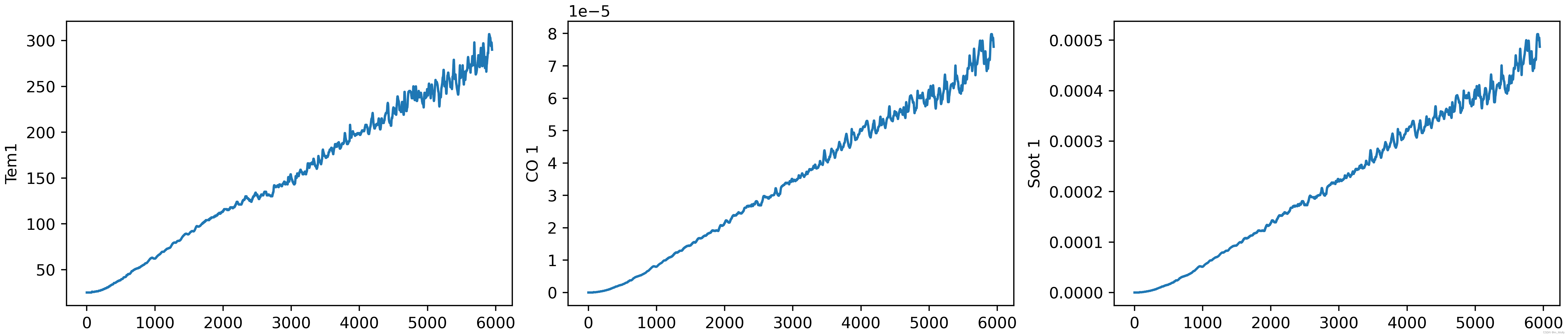
1.3 數據可視化

# 3.數據可視化 
plt.rcParams['savefig.dpi'] = 500
plt.rcParams['figure.dpi'] = 500fig,ax = plt.subplots(1,3,constrained_layout = True , figsize = (14,3))
sns.lineplot(data=df["Tem1"],ax=ax[0])
sns.lineplot(data=df["CO 1"],ax=ax[1])
sns.lineplot(data=df["Soot 1"],ax=ax[2])
plt.savefig("D:\\jupyter notebook\\DL-100-days\\RNN\\3.數據可視化.png")
#plt.show()

輸出：

二、數據預處理(構建數據集)

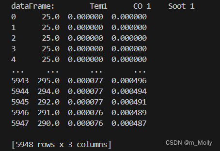
# 二、數據預處理(構建數據集)
dataFrame = df.iloc[:,1:]
print("dataFrame:", dataFrame)

輸出：

2.1 設置x、y

# 1，設置x、y
# 需要實現：使用1-8時刻段預測9時刻段，則通過下述代碼做好長度的確定：
width_X = 8
width_y = 1X = []
y = []in_start = 0for _,_ in df.iterrows():in_end = in_start + width_Xout_end = in_end + width_yif out_end < len(dataFrame):X_ = np.array(dataFrame.iloc[in_start:in_end,])X_ = X_.reshape((len(X_)*3))y_ = np.array(dataFrame.iloc[in_end:out_end,0])X.append(X_)y.append(y_)in_start += 1X = np.array(X)
y = np.array(y)print(X.shape,y.shape)

輸出：

2.2 歸一化

# 2，歸一化
from sklearn.preprocessing import MinMaxScalersc = MinMaxScaler(feature_range=(0,1))
X_scaled = sc.fit_transform(X)
print(X_scaled.shape)X_scaled = X_scaled.reshape(len(X_scaled),width_X,3)
print(X_scaled.shape)

輸出：

2.3 劃分數據集

取5000之前的數據作為訓練集，5000之后的數據作為驗證集：

# 3，劃分數據集
# 取5000之前的數據作為訓練集，5000之后的數據作為驗證集：
X_train = np.array(X_scaled[:5000]).astype('float64')
y_train = np.array(y[:5000]).astype('float64')X_test = np.array(X_scaled[5000:]).astype('float64')
y_test = np.array(y[5000:]).astype('float64')print(X_train.shape)

輸出：

三、模型創建、編譯、訓練、得到訓練結果

3.1 構建模型

通過下面代碼，構建一個包含兩個LSTM層和一個全連接層的LSTM模型。這個模型將接受形狀為(X_train.shape[1], 3)的輸入，其中X_train.shape[1]是時間步數，3 是每個時間步的特征數。

# 三、構建模型
import keras
from keras.models import Sequential
from keras.layers import Dense,LSTMmodel_lstm = Sequential()
model_lstm.add(LSTM(units=64,activation='relu',return_sequences=True,input_shape=(X_train.shape[1],3)))
model_lstm.add(LSTM(units=64,activation='relu'))
model_lstm.add(Dense(width_y))
# 通過上述代碼，構建了一個包含兩個LSTM層和一個全連接層的LSTM模型。這個模型將接受形狀為 (X_train.shape[1], 3) 的輸入，其中 X_train.shape[1] 是時間步數，3 是每個時間步的特征數。

輸出：

3.2 編譯模型

# 四、 編譯模型 
model_lstm.compile(loss='mean_squared_error',optimizer=tf.keras.optimizers.Adam(1e-3))

3.3 訓練模型

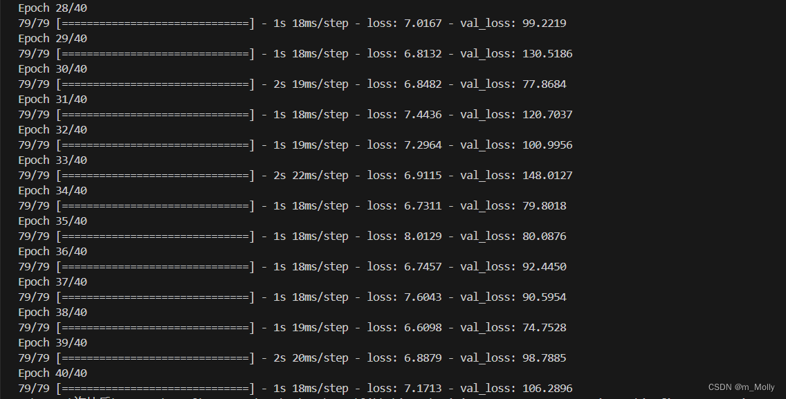
history = model_lstm.fit(X_train,y_train,epochs = 40,batch_size = 64,validation_data=(X_test,y_test),validation_freq= 1)

訓練輸出：

3.4 模型評估

3.4.1 Loss與Accuracy圖

# 六、 模型評估
# 1.Loss與Accuracy圖
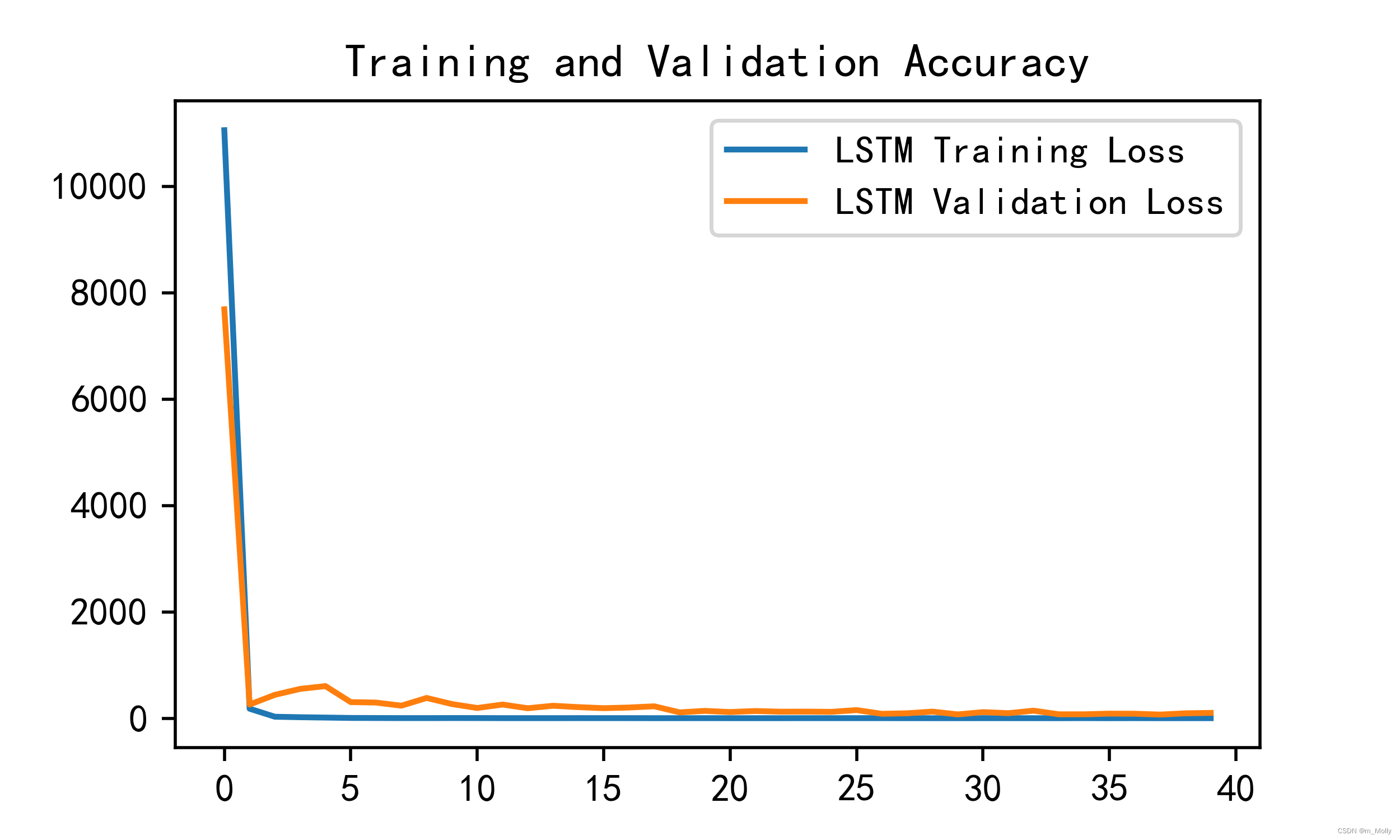
import matplotlib.pyplot as pltplt.rcParams['font.sans-serif'] = ['SimHei']
plt.rcParams['axes.unicode_minus'] = Falseplt.figure(figsize=(5, 3),dpi=120)plt.plot(history.history['loss'],label = 'LSTM Training Loss')
plt.plot(history.history['val_loss'],label = 'LSTM Validation Loss')plt.title('Training and Validation Accuracy')
plt.legend()
plt.savefig("D:\\jupyter notebook\\DL-100-days\\RNN\\1.Loss與Accuracy圖.png")
plt.show()

輸出：

3.4.2 調用模型進行預測

# 2.調用模型進行預測
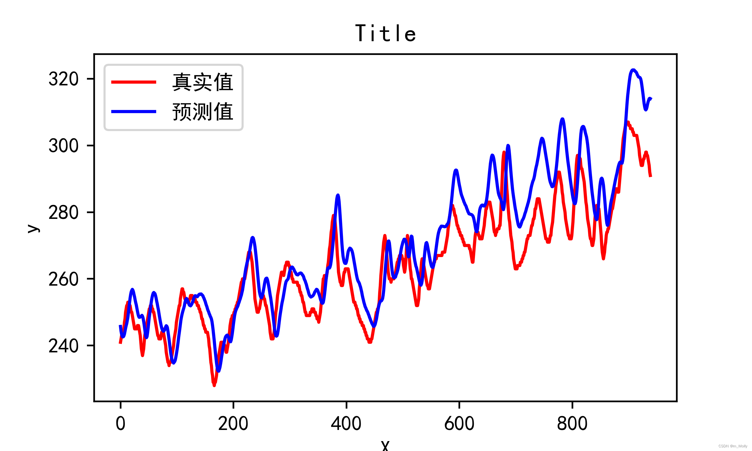
predicted_y_lstm = model_lstm.predict(X_test)y_tset_one = [i[0] for i in y_test]
predicted_y_lstm_one = [i[0] for i in predicted_y_lstm]plt.figure(figsize=(5,3),dpi=120)
plt.plot(y_tset_one[:1000],color = 'red', label = '真實值')
plt.plot(predicted_y_lstm_one[:1000],color = 'blue', label = '預測值')plt.title('Title')
plt.xlabel('X')
plt.ylabel('y')
plt.legend()
plt.savefig("D:\\jupyter notebook\\DL-100-days\\RNN\\2.調用模型進行預測圖.png")
plt.show()

輸出：

3.4.3 查看誤差

# 3. 查看誤差
from  sklearn import metricsRMSE_lstm = metrics.mean_squared_error(predicted_y_lstm,y_test)**0.5
R2_lstm = metrics.r2_score(predicted_y_lstm,y_test)print('均方根誤差：%.5f' % RMSE_lstm)
print('R2:%.5f' % R2_lstm)

輸出：

四、其他

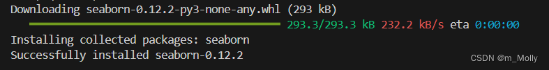
4.1 模塊報錯：seaborn模塊導入錯誤

解決方法如下：

4.2 圖片實時顯示比例不對

改為保存到本地查看：【在plt.show()之前保存】
line 34：

plt.savefig("D:\\jupyter notebook\\DL-100-days\\RNN\\3.數據可視化.png")
plt.show()

line 125：

plt.savefig("D:\\jupyter notebook\\DL-100-days\\RNN\\1.Loss與Accuracy圖.png")
plt.show()

line 143：

plt.savefig("D:\\jupyter notebook\\DL-100-days\\RNN\\2.調用模型進行預測圖.png")
plt.show()

輸出：

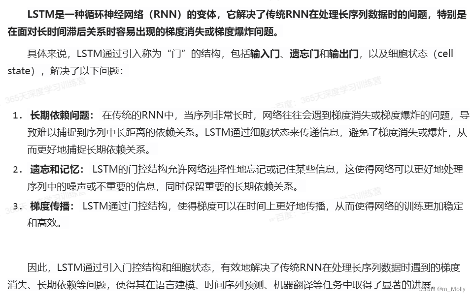
4.3 什么是LSTM

LSTM是一種特殊的RNN，能到學習到長期的依賴關系，可以理解為升級版的RNN。

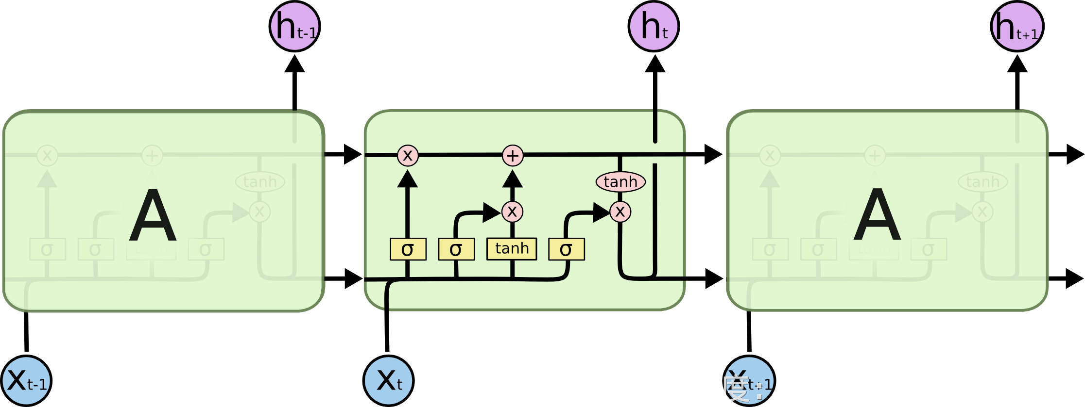
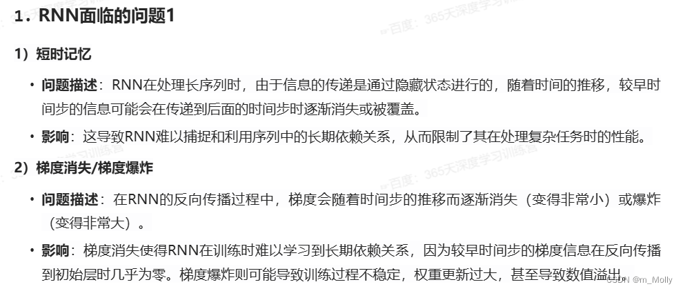
傳統的RNN在處理長序列時存在著“梯度爆炸（/梯度消失）”和“短時記憶”的問題，向RNN中加入遺忘門、輸入門及輸出門使得困擾RNN的問題得到了一定的解決；

關于LSTM的實現流程：（1、單輸出時間步）單輸入單輸出、多輸入單輸出、多輸入多輸出（2、多輸出時間步）單輸入單輸出、多輸入單輸出、多輸入多輸出；