這是一篇關于醫學數據的數據分析,但是這個數據集數據不是很多。
背景描述
本數據集包含了多個與心力衰竭相關的特征,用于分析和預測患者心力衰竭發作的風險。數據集涵蓋了從40歲到95歲不等年齡的患者群體,提供了廣泛的生理和生活方式指標,以幫助研究人員和醫療專業人員更好地理解心衰的潛在風險因素。
每條患者記錄包含以下關鍵信息:
- 年齡(Age):記錄患者的年齡,心臟病的風險隨年齡增長而增加。
- 貧血(Anaemia):貧血可能影響心臟功能,記錄患者是否患有貧血。
- 高血壓(High blood pressure):高血壓是心臟病的主要風險因素之一。
- 肌酸激酶(Creatinine phosphokinase, CPK):血液中的CPK水平可以反映心肌損傷。
- 糖尿病(Diabetes):糖尿病與心臟病風險增加有關。
- 射血分數(Ejection fraction):心臟每次收縮時泵出的血液百分比,是心臟功能的重要指標。
- 性別(Sex):性別可能影響心臟病的風險和表現形式。
- 血小板(Platelets):血小板水平可能與血液凝固和心臟病風險相關。
- 血清肌酐(Serum creatinine):血液中的肌酐水平可以反映腎臟功能,與心臟病風險有關。
- 血清鈉(Serum sodium):鈉水平的異常可能與心臟疾病相關。
- 吸煙(Smoking):吸煙是心臟病的一個重要可預防風險因素。
- 時間(Time):記錄患者的隨訪期,用于觀察長期健康變化。
- 死亡事件(death event):記錄患者在隨訪期間是否發生了死亡事件,作為研究的主要結果指標。
數據說明
| 字段 | 解釋 | 測量單位 | 區間 |
|---|---|---|---|
| Age | 患者的年齡 | 年(Years) | [40,…, 95] |
| Anaemia | 是否貧血(紅細胞或血紅蛋白減少) | 布爾值(Boolean) | 0, 1 |
| High blood pressure | 患者是否患有高血壓 | 布爾值(Boolean) | 0, 1 |
| Creatinine phosphokinase, CPK | 血液中的 CPK (肌酸激酶)水平 | 微克/升(mcg/L) | [23,…, 7861] |
| Diabetes | 患者是否患有糖尿病 | 布爾值(Boolean) | 0, 1 |
| Ejection fraction | 每次心臟收縮時離開心臟的血液百分比 | 百分比(Percentage) | [14,…, 80] |
| Sex | 性別,女性0或男性1 | 二進制(Binary) | 0, 1 |
| Platelets | 血液中的血小板數量 | 千血小板/毫升(kiloplatelets/mL) | [25.01,…, 850.00] |
| Serum creatinine | 血液中的肌酐水平 | 毫克/分升(mg/dL) | [0.50,…, 9.40] |
| Serum sodium | 血液中的鈉水平 | 毫摩爾/升(mEq/L) | [114,…, 148] |
| Smoking | 患者是否吸煙 | 布爾值(Boolean) | 0, 1 |
| Time | 隨訪期 | 天(Days) | [4,…,285] |
| DEATH_EVENT | 患者在隨訪期間是否死亡 | 布爾值(Boolean) | 0, 1 |
!pip install lifelines -i https://pypi.tuna.tsinghua.edu.cn/simple/
!pip install imblearn -i https://pypi.tuna.tsinghua.edu.cn/simple/
?這是我們這次用到的一些第三方庫,大家如果沒有安裝,可以在jupyter notebook中直接下載。
一:導入第三方庫
import pandas as pd
import numpy as np
import matplotlib.pyplot as plt
import seaborn as sns
from lifelines import KaplanMeierFitter,CoxPHFitter
import scipy.stats as stats
from sklearn.model_selection import train_test_split
from imblearn.over_sampling import RandomOverSampler
from sklearn.metrics import classification_report,confusion_matrix,roc_curve,auc
from sklearn.ensemble import RandomForestClassifier
from pylab import mplplt.rcParams['font.family'] = ['sans-serif']
plt.rcParams['font.sans-serif'] = ['SimHei']
plt.rcParams['axes.unicode_minus'] = False
?二:讀取數據
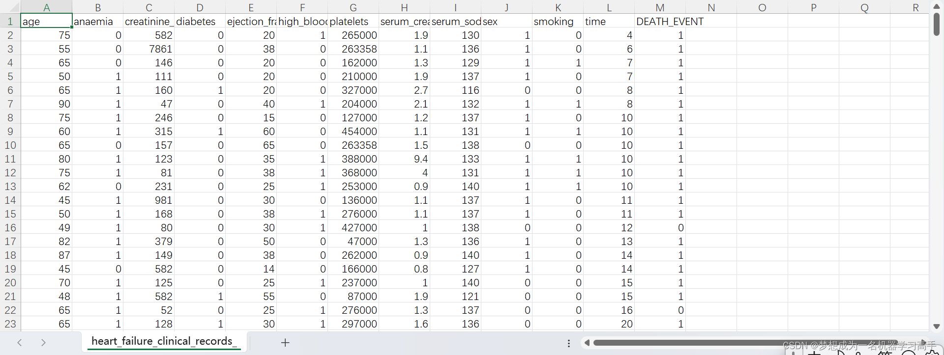
data = pd.read_csv("D:/每周挑戰/heart_failure_clinical_records_dataset.csv")
data.head()
三:對數據進行預處理
data = data.rename(columns={'age':'年齡','anaemia':'是否貧血','creatinine_phosphokinase':'血液中的CPK水平','diabetes':'患者是否患有糖尿病','ejection_fraction':'每次心臟收縮時離開心臟的血液百分比','high_blood_pressure':'患者是否患有高血壓','platelets':'血液中的血小板數量','serum_creatinine':'血液中的肌酐水平','serum_sodium':'血液中的鈉水平','sex':'性別(0為男)','smoking':'是否吸煙','time':'隨訪期(day)','DEATH_EVENT':'是否死亡'})
data.head()
# 將標簽修改為中文更好看
?上面這一段可以不寫,如果你喜歡英語可以不加,如果你喜歡漢字,那你可以更改一下。
data.info()  # 從這里可以觀察出應該是沒有缺失值
data.isnull().sum()  # 沒有缺失值
data_ = data.copy()        # 方便我們后期對數據進行建模
區分連續數據和分類數據。?
for i in data.columns:if set(data[i].unique()) == {0,1}:print(i)
print('-'*50)
for i in data.columns:if set(data[i].unique()) != {0,1}:print(i)
?四:數據分析繪圖
classify = ['anaemia','high_blood_pressure','diabetes','sex','smoking','DEATH_EVENT']  #  DEATH_EVENT 這個是研究的主要結果指標
numerical = ['age','creatinine_phosphokinase','ejection_fraction','platelets','serum_creatinine','serum_sodium','time']plt.figure(figsize=((16,20)))
for i,col in enumerate(numerical):plt.subplot(4,2,i+1)sns.boxplot(y = data[col])plt.title(f'{col}的箱線圖', fontsize=14)plt.ylabel('數值', fontsize=12)plt.grid(axis='y', linestyle='--', alpha=0.7)plt.tight_layout()
plt.show()
?從箱型圖來看,有些數據有部分異常值,但是,由于缺乏醫學知識,所以這里我們不能對異常值進行處理。
colors = ['#63FF9D', '#C191FF']
plt.figure(figsize=(10,12))
for i,col in enumerate(classify):statistics = data[col].value_counts().reset_index()plt.subplot(3,2,i+1)sns.barplot(x=statistics['index'],y=statistics[col],palette=colors)plt.title(f'{col}的條形圖', fontsize=14)plt.tight_layout()
plt.show()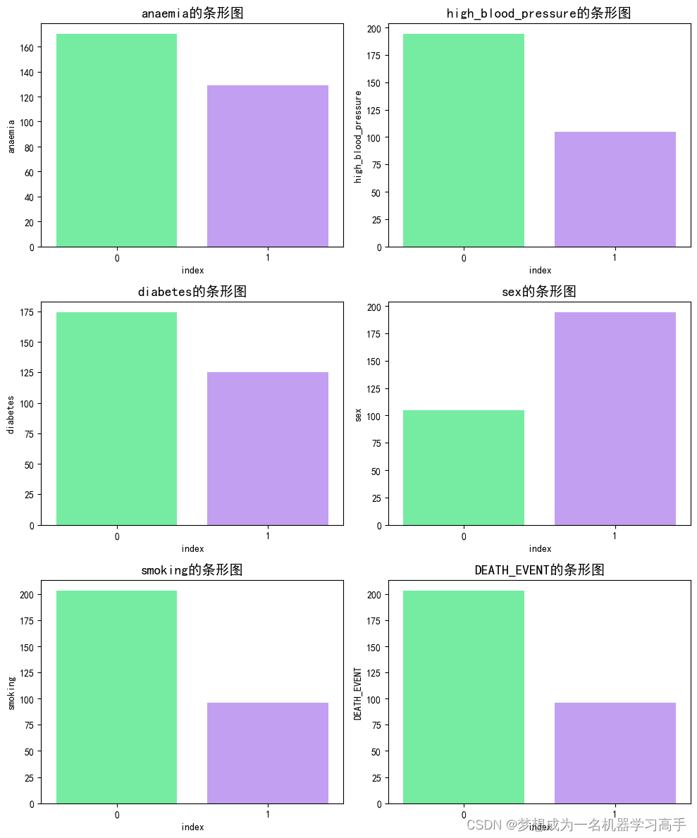
接下里,我們看時間對于生存率的影響,這里我們就用到了前面安裝的KaplanMeierFitter。
kmf = KaplanMeierFitter()
kmf.fit(durations=data['time'],event_observed=data['DEATH_EVENT'])plt.figure(figsize=(10,8))
kmf.plot_survival_function()
plt.title('Kaplan-Meier 生存曲線', fontsize=14)
plt.xlabel('時間(天)', fontsize=12)
plt.ylabel('生存概率', fontsize=12)plt.show()
隨著時間的推移,生存概率逐漸下降。 在隨訪結束時,生存概率大約為60%。 接下來,我們對特征相關性進行分析。?
corr = data.corr(method="spearman")plt.figure(figsize=(10,8))
sns.heatmap(corr,annot=True,cmap='coolwarm',fmt='.2g')
plt.title("斯皮爾曼相關性矩陣")
plt.show()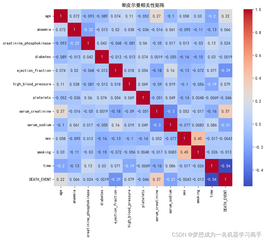
顯著相關性:
年齡、射血分數、血清肌酐 血清鈉 和 隨訪期 與死亡事件之間的相關性較強。 射血分數和血清肌酐與死亡事件的相關性尤為顯著,這表明這些變量對死亡事件的預測可能具有重要意義。 弱相關性或無相關性:
貧血、高血壓 與死亡事件有輕微相關性,但不顯著。
肌酸激酶、糖尿病、血小板、性別 和 吸煙 與死亡事件幾乎沒有相關性。
def t_test(fea):group1 = data[data['DEATH_EVENT'] == 0][fea]group2 = data[data['DEATH_EVENT'] == 1][fea]t,p = stats.ttest_ind(group1,group2)return t,p# 對數值變量進行t檢驗
t_test_results = {feature: t_test(feature) for feature in numerical}t_test_df = pd.DataFrame.from_dict(t_test_results,orient='index',columns=['T-Statistic','P-Value'])
t_test_df| T-Statistic | P-Value | |
|---|---|---|
| age | -4.521983 | 8.862975e-06 |
| creatinine_phosphokinase | -1.083171 | 2.796112e-01 |
| ejection_fraction | 4.805628 | 2.452897e-06 |
| platelets | 0.847868 | 3.971942e-01 |
| serum_creatinine | -5.306458 | 2.190198e-07 |
| serum_sodium | 3.430063 | 6.889112e-04 |
| time | 10.685563 | 9.122223e-23 |
?
t檢驗是一種統計方法,用于比較兩組數據是否存在顯著差異。該方法基于以下步驟和原理:
建立假設:首先建立零假設(H0),通常表示兩個比較群體間沒有差異,以及備擇假設(H1),即存在差異。
計算t值:計算得到一個t值,這個值反映了樣本均值與假定總體均值之間的差距大小。
確定P值:通過t分布理論,計算出在零假設為真的條件下,觀察到當前t值或更極端情況的概率,即P值。
做出結論:如果P值小于事先設定的顯著性水平(通常為0.05),則拒絕零假設,認為樣本來自的兩個總體之間存在顯著差異;否則,不拒絕零假設。
對于連續數據的特征我們采用t檢驗進行分析,而對于離散數據,我們采用卡方檢驗進行分析
# 卡方檢驗
def chi_square_test(fea1, fea2):contingency_table = pd.crosstab(data[fea1], data[fea2])chi2, p, dof, expected = stats.chi2_contingency(contingency_table)return chi2, pchi_square_results = {}
chi_square_results = {feature: chi_square_test(feature, 'DEATH_EVENT') for feature in classify}chi_square_df = pd.DataFrame.from_dict(chi_square_results,orient='index',columns=['Chi-Square','P-Value'])
chi_square_df| Chi-Square | P-Value | |
|---|---|---|
| anaemia | 1.042175 | 3.073161e-01 |
| high_blood_pressure | 1.543461 | 2.141034e-01 |
| diabetes | 0.000000 | 1.000000e+00 |
| sex | 0.000000 | 1.000000e+00 |
| smoking | 0.007331 | 9.317653e-01 |
| DEATH_EVENT | 294.430106 | 5.386429e-66 |
所有分類變量(貧血、糖尿病、高血壓、性別、吸煙)的p值均大于0.05,表明它們與死亡事件無顯著相關性。
最后我們對數據進行建模,這里我們使用隨機森林,由于數據量較少,因此我們采用隨機采樣的方法進行過采樣。
x = data.drop('DEATH_EVENT',axis=1)
y = data['DEATH_EVENT']
x_train,x_test,y_train,y_test = train_test_split(x,y,test_size=0.3,random_state=15) #37分
# 實例化隨機過采樣器
oversampler = RandomOverSampler()# 在訓練集上進行隨機過采樣
x_train, y_train = oversampler.fit_resample(x_train, y_train)rf_clf = RandomForestClassifier(random_state=15)
rf_clf.fit(x_train, y_train)y_pred_rf = rf_clf.predict(x_test)
class_report_rf = classification_report(y_test, y_pred_rf)
print(class_report_rf)
precision recall f1-score support0 0.84 0.85 0.84 601 0.69 0.67 0.68 30accuracy 0.79 90macro avg 0.76 0.76 0.76 90 weighted avg 0.79 0.79 0.79 90
cm = confusion_matrix(y_test,y_pred_rf)plt.figure(figsize=(8, 6))
sns.heatmap(cm, annot=True, fmt='g', cmap='Blues', xticklabels=['預測值 0', '預測值 1'], yticklabels=['真實值 0', '真實值 1'])
plt.title('混淆矩陣')
plt.show()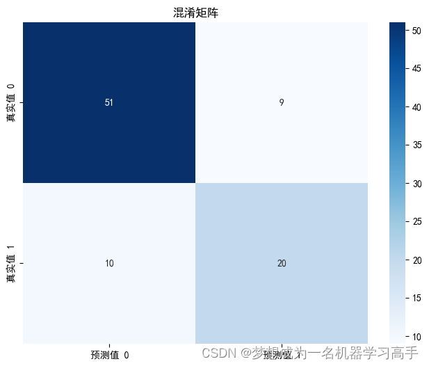
feature_importance = rf_clf.feature_importances_
feature = x.columnssort_importance = feature_importance.argsort()
plt.figure(figsize=(10,8))
plt.barh(range(len(sort_importance)), feature_importance[sort_importance],color='#B5FFCD')
plt.yticks(range(len(sort_importance)), [feature[i] for i in sort_importance])
plt.xlabel('特征重要性')
plt.title('特征重要性分析')plt.show()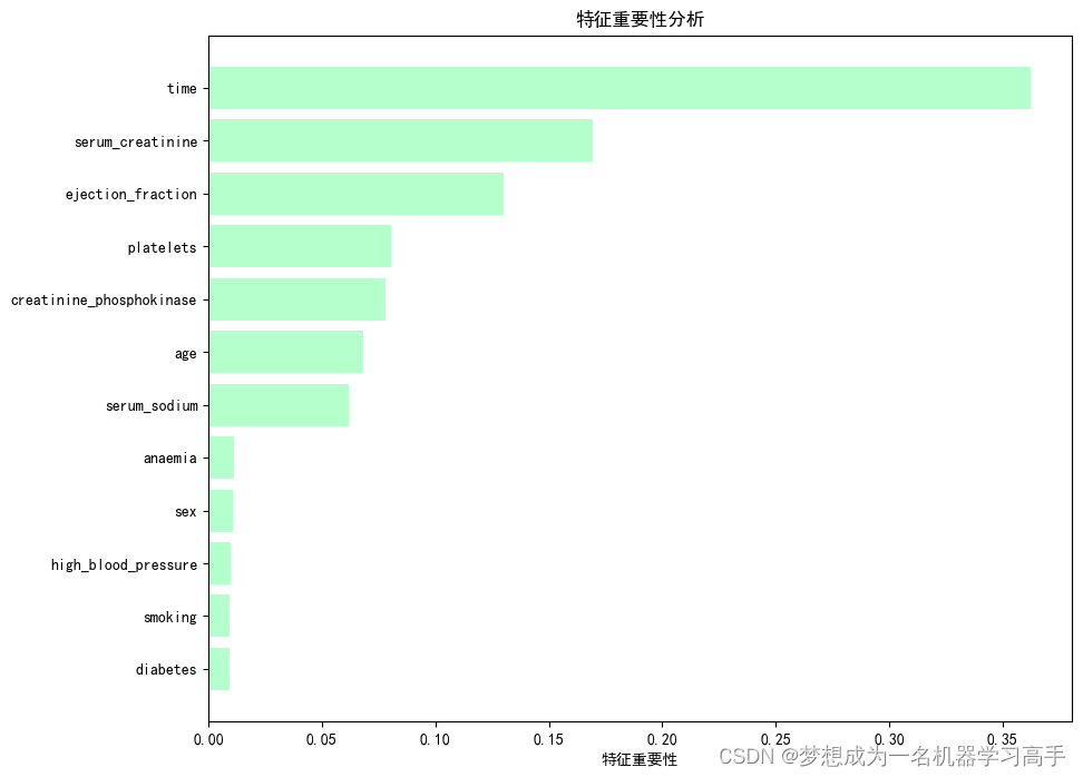


線程的同步 進程間通信)


)


)
實現)


)
