數據分析處理庫Pandas常用方法匯總

一、基礎操作

1.1 創建df對象

1.1.1 讀入表格數據

1.1.2 手動創建df

1.2 .info()

1.3 df.index

1.4 df.columns

1.5 df.dtypes

1.6 df.values

1.7?.set_index()

?1.8 df['xxx']

1.9 .describe()

1.10 .isin()

1.12 .where()

1.13?.query()

1.14?Series類型運算

二、Pandas索引結構

2.1 選擇多列?

2.2 loc / iloc

?2.3 自定義索引

?2.4 bool索引

2.5 制定多列索引?

三、數值運算操作

3.1 .sum()

3.2 .mean()

3.3 .min() / .max()

3.4?.median()

3.5?二元統計

3.5.1?df.cov()

3.5.2?df.corr()

3.5.3?.value_counts()

三、對象的增刪改查

3.1?Series結構的增刪改查

3.1.1 查操作

3.1.2 改操作

3.1.3?增操作

3.1.4?刪操作

3.2 DataFrame結構的增刪改查

3.2.1 查操作

3.2.2?改操作

3.2.3?增操作

3.2.4?刪操作

四、合并操作

4.1 .merge()

4.2 多索引合并

使用on參數?

使用how參數

4.3 join

五、數據透視表

5.1 .pivot()

5.2?.pivot_table()

六、?時間操作

6.1 創建時間序列

6.1.1. pd.to_datetime()

6.1.2. pd.date_range()

6.2 時間戳與時間區間

6.2.1. Timestamp

6.2.2. Timedelta

6.3 時間的運算與篩選

6.3.1. 時間加減

6.3.2. 篩選特定時間段

6.4 設置索引并重采樣

6.4.1. 設置時間索引

6.4.2. 取時間索引中的某個數值

6.4.3. 重采樣 resample()

6.5 時間格式的處理

6.5.1. 提取時間的各部分

6.5.2. 格式化輸出

6.6 常見時間函數總結

七、常用操作

7.1 查看數據結構與基本信息

7.1.1 df.head() / df.tail()

7.1.2 df.shape / df.columns / df.index

7.1.3 df.info() / df.describe()

7.2 數據選擇與過濾

7.2.1 選擇列

7.2.2 選擇行

7.2.3 多重條件

6.3?數據修改與添加

7.3.1 新增列

7.3.2 修改數據

7.3.3 刪除列/行

7.4 缺失值處理

7.4.1 檢查缺失值

7.4.2 刪除缺失值

7.4.3 填充缺失值

7.5. 分組與聚合

7.5.1 分組統計

單分組和多重分組

改變索引?

傳函數名的自定義分組

多索引時指定某一個索引分組

7.5.2?拆分范圍

7.5.3 一列多算

7.6. 排序與去重

7.6.1 排序

7.6.2 去重

7..7 數據合并與連接

7.7.1 拼接 concat

7.7.2 合并 merge

7.8?常見函數速查表

八、字符串操作

8.1 字符串小寫/大寫/首字母大寫

8.2 去除空格、換行等

8.3 查找與匹配字符串

8.3.1 包含判斷

8.3.2 匹配字符串開頭/結尾

8.4?替換、分割與拼接

8.4.1 替換

8.4.2 字符串分割

.str.split()

8.4.3 拼接字符串

8.5 提取子串與正則提取

8.5.1 提取固定位置子串

8.5.2 正則提取

8.6 字符串長度統計

8.7?.get_dummies()

8.8?常用字符串函數速查表

一、基礎操作

Series：

一維數據結構，類似于一個帶索引的數組。

每個元素都有一個對應的索引值，索引是唯一的。

通常用于表示單列數據。

通過一個列表、數組或字典創建。

DataFrame：

二維數據結構，類似于一個表格，由行和列組成。

每列可以有不同的數據類型（如整數、浮點數、字符串等）。

每行和每列都有索引，行索引稱為 index，列索引稱為 columns。

通常用于表示多列數據。

通過字典、列表的列表、或從文件（如 CSV、Excel）中讀取創建。

1.1 創建df對象

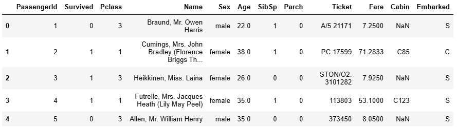
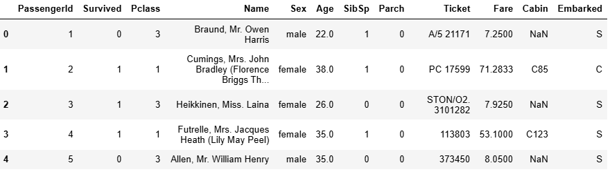
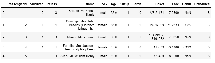
1.1.1 讀入表格數據

df = pd.read_csv('./data/titanic.csv')
df.head() #可以讀前5行數據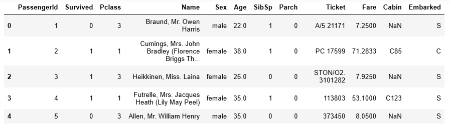

1.1.2 手動創建df

data = {'country':['aaa','bbb','ccc'],'population':[10,12,14]}
df_data = pd.DataFrame(data)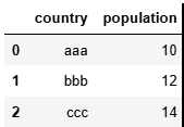

1.2 .info()

返回當前的信息

df.info()輸出：<class 'pandas.core.frame.DataFrame'>
RangeIndex: 891 entries, 0 to 890
Data columns (total 12 columns):#   Column       Non-Null Count  Dtype  
---  ------       --------------  -----  0   PassengerId  891 non-null    int64  1   Survived     891 non-null    int64  2   Pclass       891 non-null    int64  3   Name         891 non-null    object 4   Sex          891 non-null    object 5   Age          714 non-null    float646   SibSp        891 non-null    int64  7   Parch        891 non-null    int64  8   Ticket       891 non-null    object 9   Fare         891 non-null    float6410  Cabin        204 non-null    object 11  Embarked     889 non-null    object 
dtypes: float64(2), int64(5), object(5)
memory usage: 83.7+ KB

1.3 df.index

返回索引對象

RangeIndex(start=0, stop=891, step=1)

1.4 df.columns

返回 DataFrame 的列名

Index(['PassengerId', 'Survived', 'Pclass', 'Name', 'Sex', 'Age', 'SibSp','Parch', 'Ticket', 'Fare', 'Cabin', 'Embarked'],dtype='object')

1.5 df.dtypes

返回 DataFrame 中每列的數據類型

PassengerId      int64
Survived         int64
Pclass           int64
Name            object
Sex             object
Age            float64
SibSp            int64
Parch            int64
Ticket          object
Fare           float64
Cabin           object
Embarked        object
dtype: object

1.6 df.values

返回 DataFrame 中的數據部分，以二維數組（NumPy 數組）的形式。

array([[1, 0, 3, ..., 7.25, nan, 'S'],[2, 1, 1, ..., 71.2833, 'C85', 'C'],[3, 1, 3, ..., 7.925, nan, 'S'],...,[889, 0, 3, ..., 23.45, nan, 'S'],[890, 1, 1, ..., 30.0, 'C148', 'C'],[891, 0, 3, ..., 7.75, nan, 'Q']], dtype=object)

1.7?.set_index()

自己指定索引

df = df.set_index('Name')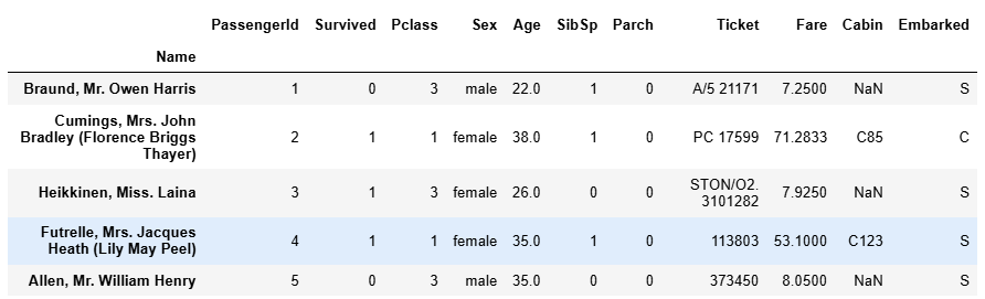

?1.8 df['xxx']

xxx表示列名，返回Series類型

age = df['Age']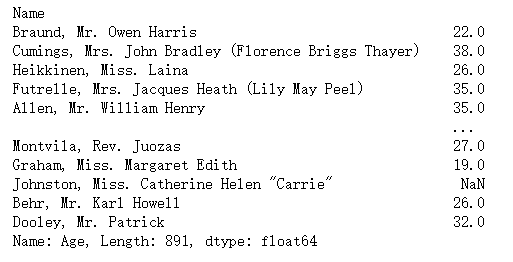

1.9 .describe()

可以得到數據的基本統計特性

df.describe()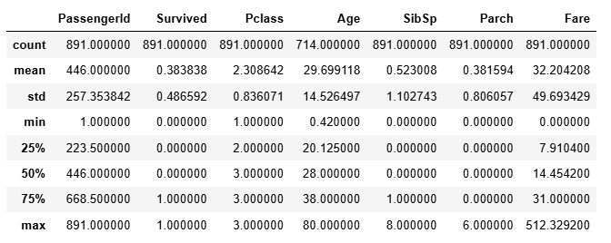

1.10 .isin()

判斷元素是否在給定內容中

s.isin([1,3,4])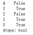

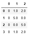
1.12 .where()

保留滿足條件的數據，替換不滿足條件的數據

df.where(df < 0)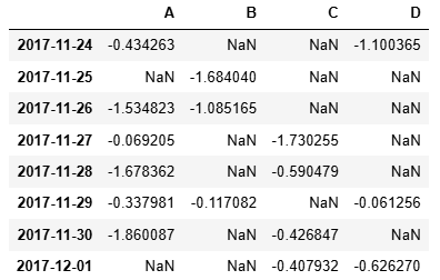

df.where(df < 0,999) #將大于0的數全部替換為999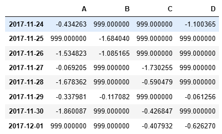

1.13?`.query()`

用于通過字符串表達式對 DataFrame 進行條件篩選?

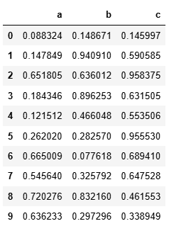
df.query('(a<b) & (b<c)')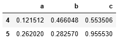

1.14?Series類型運算

.mean() / .max() / .min()，廣播+-*%

age = age + 10
age.mean()
age.max()
age.min()

二、Pandas索引結構

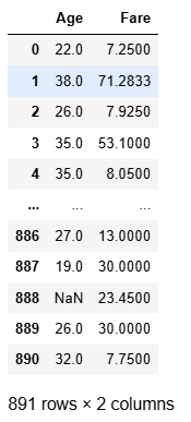
2.1 選擇多列?

df[['Age','Fare']]

2.2 loc / iloc

loc 用label來去定位
iloc 用position來去定位

df.iloc[0:5]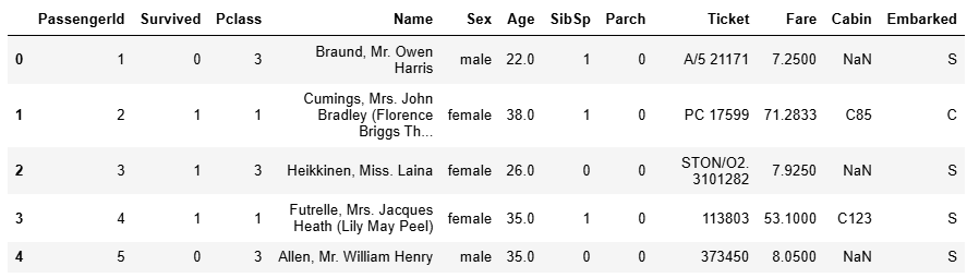

df.iloc[0:2]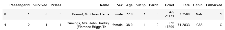

?2.3 自定義索引

df = df.set_index('Name')
df.loc['Heikkinen, Miss. Laina']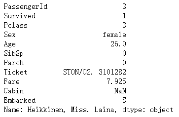

也支持切片操作

df.loc['Heikkinen, Miss. Laina':'Allen, Mr. William Henry']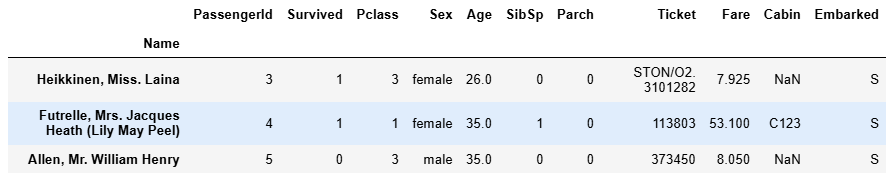

?2.4 bool索引

df[df['Fare'] > 40][0:5]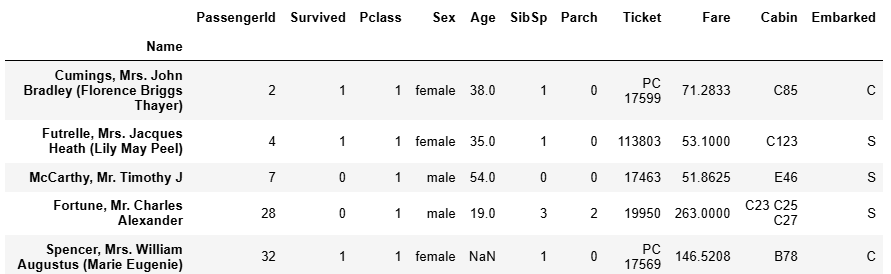

?下邊兩種寫法相同

df.loc[df['Sex'] == 'male'][['Fare','Age']]
df.loc[df['Sex'] == 'male',['Fare','Age']]

2.5 制定多列索引?

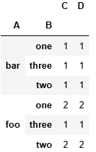
s2 = pd.Series(np.arange(6),index = pd.MultiIndex.from_product([[0,1],['a','b','c']]))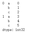

三、數值運算操作

創建DataFrame

df = pd.DataFrame([[1,2,3],[4,5,6]],index = ['a','b'],columns = ['A','B','C'])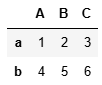

3.1 .sum()

默認axis=0

3.2 .mean()

默認axis=0

3.3 .min() / .max()

默認axis=0

3.4?.median()

默認axis=0

3.5?二元統計

3.5.1?df.cov()

計算 DataFrame 中各列之間的協方差矩陣。

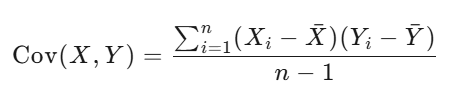
df.cov()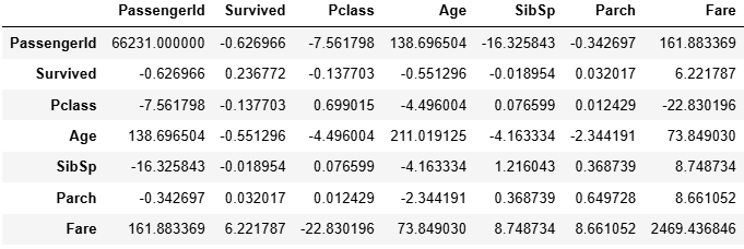

3.5.2?df.corr()

計算 DataFrame 中各列之間的相關系數矩陣。

df.corr()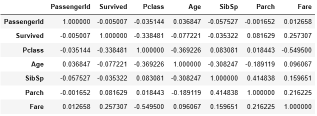

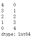
3.5.3?.value_counts()

統計元組數量

df['Age'].value_counts()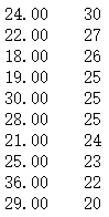

df['Age'].value_counts(ascending = True)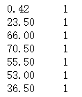

三、對象的增刪改查

3.1?Series結構的增刪改查

data = [10,11,12]
index = ['a','b','c']
s = pd.Series(data = data,index = index)

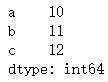
3.1.1 查操作

s[0]  --> 10
s[0:2]
mask = [True,False,True]
s[mask]
s.loc['b'] --> 11
s.iloc[1] --> 11

3.1.2 改操作

s1['a'] = 100
s1.replace(to_replace = 100,value = 101,inplace = False)

inplace表示是否要在s1上修改

修改index

s1.index = ['a','b','d']
s1.rename(index = {'a':'A'},inplace = True)

3.1.3?增操作

data = [100,110]
index = ['h','k']
s2 = pd.Series(data = data,index = index)輸出：
h    100
k    110
dtype: int64

.concat([xx,xx])?

s3 = pd.concat([s1,s2])輸出：
A    101
b     11
c     12
h    100
k    110
dtype: int64pd.concat([s1,s2],ignore_index = True)輸出：
0    101
1     11
2     12
3    100
4    110
dtype: int64

?直接新增新索引

s3['j'] = 500輸出：
A    101
b     11
c     12
h    100
k    110
j    500
dtype: int64

3.1.4?刪操作

del s1['A']
s1.drop(['b','d'],inplace = True)

3.2 DataFrame結構的增刪改查

data = [[1,2,3],[4,5,6]]
index = ['a','b']
columns = ['A','B','C']df = pd.DataFrame(data=data,index=index,columns = columns)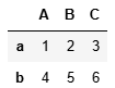

3.2.1 查操作

df['A']
輸出：
a    1
b    4
Name: A, dtype: int64

df.iloc[0]
df.loc['a']

3.2.2?改操作

df.loc['a','A'] --> 1
df.loc['a']['A'] = 150

3.2.3?增操作

df.loc['c'] = [1,2,3]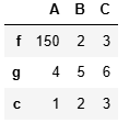

df3 = pd.concat([df,df2],axis = 0)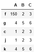

df2['Tang'] = [10,11]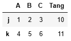

3.2.4?刪操作

df5.drop(['j'],axis=0,inplace = True) --> 去除1行
df5.drop(['A','B','C'], axis = 1,inplace = True) --> 去除多列
del df5['Tang'] --> 去除1列

四、合并操作

left = pd.DataFrame({'key': ['K0', 'K1', 'K2', 'K3'],'A': ['A0', 'A1', 'A2', 'A3'], 'B': ['B0', 'B1', 'B2', 'B3']})
right = pd.DataFrame({'key': ['K0', 'K1', 'K2', 'K3'],'C': ['C0', 'C1', 'C2', 'C3'], 'D': ['D0', 'D1', 'D2', 'D3']})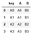

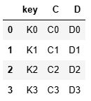
4.1 .merge()

res = pd.merge(left, right)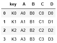

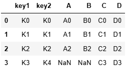
4.2 多索引合并

left = pd.DataFrame({'key1': ['K0', 'K1', 'K2', 'K3'],'key2': ['K0', 'K1', 'K2', 'K3'],'A': ['A0', 'A1', 'A2', 'A3'], 'B': ['B0', 'B1', 'B2', 'B3']})
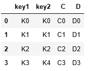
right = pd.DataFrame({'key1': ['K0', 'K1', 'K2', 'K3'],'key2': ['K0', 'K1', 'K2', 'K4'],'C': ['C0', 'C1', 'C2', 'C3'], 'D': ['D0', 'D1', 'D2', 'D3']})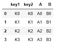

使用on參數?

res = pd.merge(left,right,on='key1')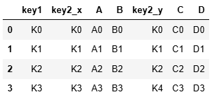

res = pd.merge(left, right, on = ['key1', 'key2'])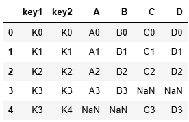

使用how參數

outer為并集

res = pd.merge(left, right, on = ['key1', 'key2'], how = 'outer', indicator = True)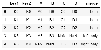

left按照左合并，right按照右合并

res = pd.merge(left, right, how = 'left')
res = pd.merge(left, right, how = 'right')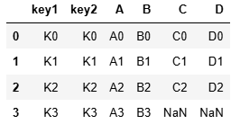

4.3 join

left = pd.DataFrame({'A': ['A0', 'A1', 'A2', 'A3'],'B': ['B0', 'B1', 'B2', 'B3'],'key': ['K0', 'K1', 'K0', 'K1']})
right = pd.DataFrame({'C': ['C0', 'C1'],'D': ['D0', 'D1']},index=['K0', 'K1'])

result = left.join(right, on='key')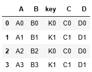

五、數據透視表

import pandas as pd
example = pd.DataFrame({'Month': ["January", "January", "January", "January", "February", "February", "February", "February", "March", "March", "March", "March"],'Category': ["Transportation", "Grocery", "Household", "Entertainment","Transportation", "Grocery", "Household", "Entertainment","Transportation", "Grocery", "Household", "Entertainment"],'Amount': [74., 235., 175., 100., 115., 240., 225., 125., 90., 260., 200., 120.]})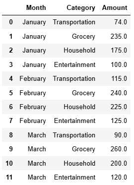

5.1 .pivot()

example_pivot = example.pivot(index = 'Category',columns= 'Month',values = 'Amount')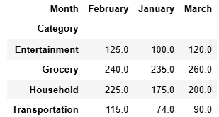

求和

example_pivot.sum(axis = 0)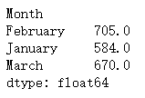

5.2?.pivot_table()

默認求均值

df.pivot_table(index = 'Sex',columns='Pclass',values='Fare')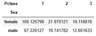

aggfunc參數定義求法

df.pivot_table(index = 'Sex',columns='Pclass',values='Fare',aggfunc='max')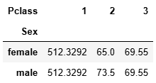

計數

df.pivot_table(index = 'Sex',columns='Pclass',values='Fare',aggfunc='count')
pd.crosstab(index = df['Sex'],columns = df['Pclass']) #計數，同上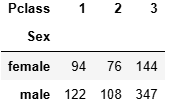

六、?時間操作

6.1 創建時間序列

6.1.1. `pd.to_datetime()`

將字符串或其他格式轉換為 datetime64[ns] 類型。

pd.to_datetime('2023-04-01')
pd.to_datetime(['2023-01-01', '2023-02-01'])

6.1.2. `pd.date_range()`

創建固定頻率的時間序列。

pd.date_range(start='2023-01-01', end='2023-01-10', freq='D')

常用頻率參數包括：

'D'：日

'H'：小時

'M'：月

'Y'：年

'W'：周

6.2 時間戳與時間區間

6.2.1. `Timestamp`

單個時間點，Pandas 對 datetime 的封裝：

ts = pd.Timestamp('2023-01-01 12:00:00')
ts.year  # 2023
ts.month # 1

6.2.2. `Timedelta`

表示時間間隔：

delta = pd.Timedelta('2 days 3 hours')

也可以進行加減操作：

pd.Timestamp('2023-01-01') + pd.Timedelta(days=3)

6.3 時間的運算與篩選

6.3.1. 時間加減

df['new_date'] = df['date'] + pd.Timedelta(days=7)

6.3.2. 篩選特定時間段

df[(df['date'] >= '2023-01-01') & (df['date'] <= '2023-03-01')]

6.4 設置索引并重采樣

6.4.1. 設置時間索引

df.set_index('date', inplace=True)

6.4.2. 取時間索引中的某個數值

data[data.index.month == 1]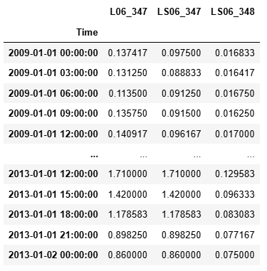

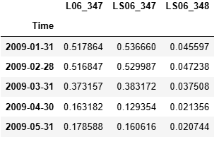
6.4.3. 重采樣 `resample()`

將數據按時間頻率重新分組，常用于聚合、統計：

df.resample('M').mean()  # 按月取平均
df.resample('W').sum()   # 按周求和

6.5 時間格式的處理

6.5.1. 提取時間的各部分

df['date'].dt.year
df['date'].dt.month
df['date'].dt.weekday

6.5.2. 格式化輸出

df['date'].dt.strftime('%Y-%m-%d')

6.6 常見時間函數總結

函數名	作用
`pd.to_datetime()`	轉換為日期時間格式
`pd.date_range()`	創建規則時間序列
`.dt.year/.month/...`	提取時間字段
`pd.Timedelta()`	表示時間間隔
`.resample()`	重采樣
`.strftime()`	時間格式化為字符串

七、常用操作

7.1 查看數據結構與基本信息

7.1.1 `df.head()` / `df.tail()`

查看前幾行或后幾行數據：

df.head(5)
df.tail(3)

7.1.2 `df.shape` / `df.columns` / `df.index`

快速了解數據的行列信息：

df.shape     # 返回 (行數, 列數)
df.columns   # 返回列名
df.index     # 返回索引

7.1.3 `df.info()` / `df.describe()`

了解字段類型和統計信息：

df.info()       # 查看每列數據類型和非空數量
df.describe()   # 查看數值列統計信息

7.2 數據選擇與過濾

7.2.1 選擇列

df['列名']
df[['列1', '列2']]

7.2.2 選擇行

df.iloc[0]           # 按位置
df.loc[0]            # 按標簽
df[df['列'] > 100]   # 條件篩選

7.2.3 多重條件

df[(df['A'] > 10) & (df['B'] < 5)]

6.3?數據修改與添加

7.3.1 新增列

df['新列'] = df['A'] + df['B']

7.3.2 修改數據

df.loc[0, 'A'] = 999

7.3.3 刪除列/行

df.drop('列名', axis=1)         # 刪除列
df.drop([0, 1], axis=0)        # 刪除行

7.4 缺失值處理

7.4.1 檢查缺失值

df.isnull()

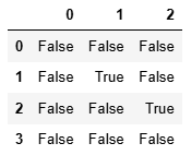
df.isnull().any(axis=0)

7.4.2 刪除缺失值

df.dropna()

7.4.3 填充缺失值

df.fillna(5)
df.fillna(method='ffill')  # 前向填充

7.5. 分組與聚合

7.5.1 分組統計

單分組和多重分組

df.groupby('列名').sum()
df.groupby('列名')['目標列'].mean()

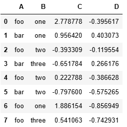
grouped = df.groupby('A')
grouped.count()grouped = df.groupby(['A','B'])
grouped.count()

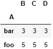
改變索引?

grouped = df.groupby(['A','B'],as_index = False)
grouped.aggregate(np.sum)#上下等價df.groupby(['A','B']).sum().reset_index()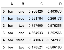

傳函數名的自定義分組

def get_letter_type(letter):if letter.lower() in 'aeiou':return 'a'else:return 'b'
grouped = df.groupby(get_letter_type,axis = 1)
grouped.count()

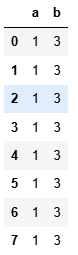
多索引時指定某一個索引分組

level=0表示第一個索引，level=1表示第一個索引，以此類推

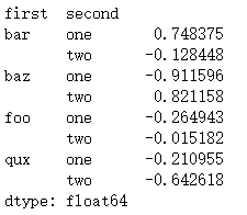
grouped = s.groupby(level =0) #或寫為level='first'
grouped.sum()

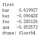
7.5.2?拆分范圍

?根據bins中給定的范圍將ages內容拆分到(10,40],(40,80]內

ages = [15,18,20,21,22,34,41,52,63,79]
bins = [10,40,80]
bins_res = pd.cut(ages,bins)

7.5.3 一列多算

使用.agg([xx,xx,xx])

grouped = df.groupby('A')
grouped['C'].agg([np.sum,np.mean,np.std])
#上下等價
grouped['C'].agg(['sum','mean','std'])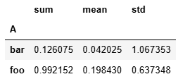

列重命名

grouped['C'].agg(res_sum=np.sum,res_mean='mean',res_std='std')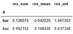

7.6. 排序與去重

7.6.1 排序

df.sort_values(by='列名', ascending=False)

7.6.2 去重

df.drop_duplicates()

7..7 數據合并與連接

7.7.1 拼接 concat

pd.concat([df1, df2], axis=0)  # 行拼接
pd.concat([df1, df2], axis=1)  # 列拼接

7.7.2 合并 merge

pd.merge(df1, df2, on='key')               # 內連接
pd.merge(df1, df2, how='left', on='key')   # 左連接

7.8?常見函數速查表

操作分類	函數	說明
查看數據	`head()` / `info()`	查看基本信息
選擇數據	`iloc` / `loc`	按位置或標簽選取
缺失值	`isnull()` / `fillna()`	檢查與填充缺失值
分組	`groupby()` / `agg()`	聚合運算
合并拼接	`merge()` / `concat()`	數據合并
應用函數	`apply()` / `lambda`	自定義處理

八、字符串操作

通過 .str 接口完成

8.1 字符串小寫/大寫/首字母大寫

df['列名'].str.lower()     # 全部轉小寫
df['列名'].str.upper()     # 全部轉大寫
df['列名'].str.title()     # 每個單詞首字母大寫

8.2 去除空格、換行等

df['列名'].str.strip()      # 去除首尾空格
df['列名'].str.lstrip()     # 去除左側空格
df['列名'].str.rstrip()     # 去除右側空格

也可處理特殊字符，如換行符 \n：

df['列名'].str.replace('\n', '')

8.3 查找與匹配字符串

8.3.1 包含判斷

df['列名'].str.contains('關鍵詞')

例如：?

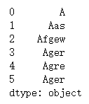
s[s.str.contains('Ag')]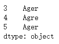

可添加正則與忽略大小寫：

df['列名'].str.contains('abc', case=False, regex=True)

8.3.2 匹配字符串開頭/結尾

df['列名'].str.startswith('前綴')
df['列名'].str.endswith('后綴')

8.4?替換、分割與拼接

8.4.1 替換

df['列名'].str.replace('舊', '新', regex=False)

也支持正則替換：

df['列名'].str.replace('\d+', '', regex=True)  # 去除所有數字

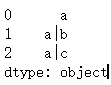
8.4.2 字符串分割

.str.split()

舉例：?

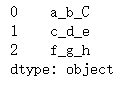
s.str.split('_')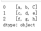

s.str.split('_',expand = True)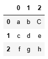

s.str.split('_',expand = True,n=1) #n=1表示切1次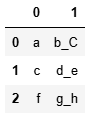

8.4.3 拼接字符串

df['新列'] = df['列A'] + '-' + df['列B']

注意拼接前需轉換為字符串：

df['列A'].astype(str) + df['列B']

8.5 提取子串與正則提取

8.5.1 提取固定位置子串

df['列名'].str[0:4]     # 提取前4位
df['列名'].str[-2:]     # 提取最后2位

8.5.2 正則提取

df['列名'].str.extract('(\d{4})')  # 提取年份

8.6 字符串長度統計

df['列名'].str.len()

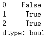
8.7?.get_dummies()

用于將字符串數據轉換為虛擬變量（one-hot 編碼）。這種方法特別適合處理包含多個分類標簽的字符串數據

s.str.get_dummies(sep = '|')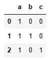

1表示該行有此字母，0表示該行沒有此字母

8.8?常用字符串函數速查表

操作類型	方法	示例
大小寫轉換	`str.lower()`	轉小寫
去空格	`str.strip()`	去首尾空格
查找包含	`str.contains('a')`	包含判斷
替換字符	`str.replace('a','b')`	替換字符串
分割	`str.split('-')`	按分隔符切分
拼接	`列1 + '-' + 列2`	拼接列
提取	`str.extract('正則')`	提取內容
統計長度	`str.len()`	計算字符串長度
獲取one-hot	`str.`get_dummies()	得到對應one-hot值