格蘭杰和格蘭杰因果

網絡搜到的Grange大神標準照

格蘭杰1934年9月出生于英國威爾士的斯旺西，早期就讀于諾丁漢大學，接受當時英國第一個經濟學數學雙學位教育，1955年留校任教，1957年在天文學雜志上他發表了第一篇論文：“關于太陽黑子活動的一個統計模型”。1959年，他在諾丁漢大學獲得統計學博士學位。在20世紀60年代早期，格蘭杰獲得了支持英國學者去美國深造的哈克尼斯(Harkness)獎學金，去普林斯頓做訪問學者，在著名學者約翰·塔基(John Tukey)和奧斯卡·摩根斯坦(Oscar Morgenstein)門下深造。1974年移居美國,成為圣迭亞哥加州大學經濟學院教授。隨后,他開創了該學院的計量經濟學研究工作,并使之成為全世界最出色的計量經濟學研究基地之一。最后成為該校的榮譽退休教授。格蘭杰于1991年成為國際預測師協會會員，曾獲得斯德哥爾摩經濟學院和卡洛斯三世大學的榮譽博士學位。他現為西部經濟學會主席、每年僅兩位的美國經濟學會杰出會員。他的研究興趣主要在統計學和計量經濟學(主要是時間序列分析)、預測、金融、人口統計學和方法論等方面。

2003年諾貝爾經濟學獎獲得者，克萊夫·格蘭杰，2003年諾貝爾經濟學獎得主，來自美國加州大學圣迭戈分校。克萊夫·格蘭杰(Clive W.J. Granger)教授因“協整理論”在時間序列數據分析上做出的杰出貢獻而獲2003年諾貝爾經濟學獎。

經濟學家開拓了一種試圖分析變量之間的格蘭杰因果關系的辦法，即格蘭杰因果關系檢驗。該檢驗方法為2003年諾貝爾經濟學獎得主克萊夫·格蘭杰(Clive W. J. Granger)所開創，用于分析經濟變量之間的格蘭杰因果關系。他給格蘭杰因果關系的定義為“依賴于使用過去某些時點上所有信息的最佳最小二乘預測的方差。

格蘭杰教授被認為是世界上最偉大的計量經濟學家之一，瑞典皇家科學院曾說，“他不僅是研究員們學習的光輝典范，而且也是金融分析家的楷模。”無數經濟學專業的學生奮斗一生，也只是為了能遠遠看到他的背影。他在利用數學模型分析時間序列數據方面的實證研究，給全世界打開了一扇窺探經濟運行規律，特別是金融市場運行規律的大門。正因如此，我們可以對股市和匯市浩如煙海的數據進行分析整理，并預測今后的走勢。

從訪問普林斯頓的20世紀60年代早期開始，格蘭杰就是一位非常有影響的時間序列計量經濟學學者。他的論文幾乎涵蓋了過去40年間該領域的主要進展，沒有格蘭杰的分析方法，進行時間序列計量方面的實證分析幾乎是不可能的。就他所產生的學術影響，人們對他的嘆服可以用天才的研究者和作家來表達。

格蘭杰的學術作品有兩個突出的特點，學術思想與實際問題密切相關；很強的可讀性，因此很多內容已經成為引用的經典。也許，這些方面的長處除了與他本人的天才資質有關之外，還和他的學習經歷有關。早在讀高中時，他就曾在兩個語法學校就讀。而且他喜歡純粹的數學思維訓練，在初學經濟學時，就對當時只會純文字描述的經濟學家感到遺憾。

諾貝爾獎評委會認為，格蘭杰的工作改變了經濟學家處理時間序列數據的方法，對研究財富與消費、匯率與價格、以及短期利率與長期利率之間的關系具有非常重要意義。目前美國聯邦儲備委員會和許多國家的中央銀行都使用這一方法來進行評估和預測。

混頻數據的計量經濟學方法

這里簡要回顧處理混頻數據的計量經濟學模型。

典型的計量經濟學回歸方程處理的是具有相同采樣頻率的變量。為保持頻率相同，研究人員要么將高頻觀測值加總為最低頻率數據，要么對低頻數據進行插值以得到最高頻率數據。在實證應用中，前者為最常用的方法，高頻數據通過平均或者取一個代表值(例如每個季度的最后一個月)而將為最低頻率。這種對數據進行“預過濾”而使得預測方程左側和右側變量成為同頻率的方法有一個潛在的問題，就是可能會破壞高頻數據中大量的有用信息。因此，對混頻數據進行直接建模是十分必要的。

這里，我稍微直白來講講，簡單講，假設你原來構建的是季度模型，例如用到了GDP增速季度數據，假設用CPI測度通脹率，而CPI數據有月度數據，傳統的做法，就是將月度CPI通過一定的算法(折騰)調整為季度數據，在數據頻率轉換的過程中，自然會損失很多信息，也有很大的爭議，月度CPI時間序列轉為季度CPI時間序列，十個人可能有十五種結果。混頻數據建模技術出現之后，就不用走這個步驟了，直接拿月度CPI和季度GDP建模就是。

混頻數據的計量經濟學應用研究很廣泛，例如

1 橋接方程

2 混頻數據取樣(MIDAS)方法，包括MIDAS權重函數，AR-MIDAS模型，CoMIDAS模型，及其拓展等等。

3 混頻－向量自回歸(MF-VAR)模型

4 混頻因子模型， 包括混頻小規模因子模型、混頻大規模因子模型，混頻狀態空間

5 因子-MIDAS模型，包括平滑因子—MIDAS模型，無限制因子—MIDAS模型

6 粗糙邊緣數據預測的實時預測

7 NowCasting等等

8 還有我想起來的混頻-GARCH模型

混頻數據格蘭杰因果檢驗的簡要數學形式

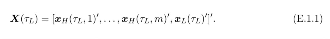
疊加的高頻(HF)和低頻(LF)變量為：

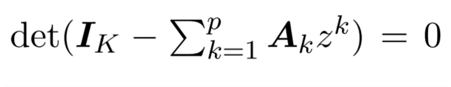
假設1： X(L) 是VAR(p)

假設2：多項式的所有根在單位圓之外

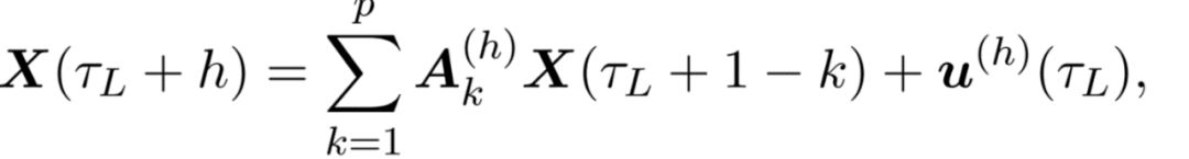
假設3：(p,h)自回歸

協方差矩陣性質：

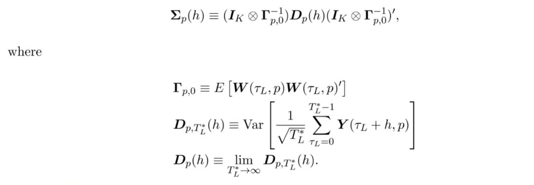
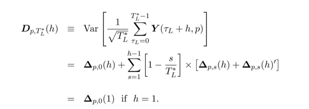
Dp(h)推導：

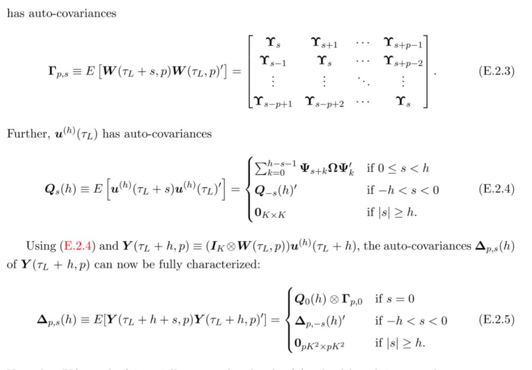
Tau和Delta p,s(h)推導：

實例的Matlab主程序(注解很清晰)

%%%%%%%% Ten requiredcodes in order to run this main code %%%%%%%%%%%%%%%%%%%%%%%

% 1. VAR_est1.m: Fit(p,h)-autoregression (i.e. VAR(p) model iterated h-times)

%??????????????? with Newey and West's (1987)HAC estimator. Newey and West's (1994)

%??????????????? automatic bandwidth selectionis available.

% 2. irf3.m: Computeimpulse response function at horizon 0, 1, ..., hmax

%??????????? along with bootstrapped confidenceintervals.

%??????????? Cholesky decomposition is used.

% 3. var_decomp.m:Forecast error variance decomposition at horizon 0, ..., hmax-1.

%????????????????? Cholesky decomposition isused.

% 4. MFCTGK_all1.m:Implement bilateral mixed frequency Granger causality tests

%?????????????????? for all possible pairs.

% 5. CTGK_all1.m:Implement bilateral Granger causality tests for all

%???????????????? possible pairs.

% 6. sim_VAR.m: SimulateVAR(p) processes.

% 7. sim_phauto.m:Simulate (p,h)-autoregression (i.e. VAR(p) iterated h-times)

% 8.causality_test_GK4.m: Implement Granger causality tests.

%????????????????????????? Goncalves andKillian's (2004) bootstrap is available.

% 9.mf_causal_test_GK4.m: Implement mixed frequency Granger causality tests.

%????????????????????????? Goncalves andKillian's (2004) bootstrap is available.

% 10. Wald_test.m:Implement Wald tests.

%%%%%%%%%%%%%%%%%%%%%%%%%%%%%%%%%%%%%%%%%%%%%%%%%%%%%%%%%%%%%%%%%%%%%%%%%%%%%%%%%%%%

%% Scenario

% We analyze threevariables x, y, z.

% x is a monthly variablewhile y and z are quarterly variables.

% The ratio of samplingfrequencies, m, is equal to 3.

% construct a 5 x 1 mixedfrequency vector X = [x1, x2, x3, y, z]'.

% Assume DGP is MF-VAR(1)with coefficient:

A = [?? 0,??0.1,?? 0.4,??? 0,???0;

????? 0.1,?-0.1,?? 0.2,??? 0,???0;

??????? 0,????0,?? 0.1,??? 0,???0;

????? 0.0,?-0.9,?? 0.9,? 0.2,???0;

??????? 0,????0,???? 0,? 0.9,?0.6];

% Evidently, (1) x causesy and (2) y causes z.

% See A(4, 1:3) for (1)and A(5,4) for (2).

% Let's generate datafrom this DGP and fit MF-VAR(1) to see what happens.

%% Step 1: Initialsetting

% general setting

T = 80;??????????? % sample size is 80 quarters, a realistic size.

m = 3; ????????????% ratio of sampling frequencies (month vs. quarter)

K_H = 1;?????????? % one high frequency variable x

K_L = 2;?????????? % two low frequency variables y, z

K = K_L + m*K_H;?? %dimension of MF-VAR

p = 1;???????????? % VAR lag length included.

?????????????????? % true lag order is 1.

lambda = 'NW';???? % useNewey and West's (1994) automatic bandwidth selection

% Impulse responsefunctions

irfhmax = 6;?????? % maximum horizon

figureflag = 1;??? % drawfigure

irfalpha = 0.05;?? % draw95% bootstrapped confidence interval

bsnum = 500;?????? % # of bootstrap replications

labels = char('x1', 'x2', 'x3', 'y', 'z');? %labels

% forecast error variancedecomposition

vdhmax = 6;??????? % maximum horizon

% Granger causality tests

gcbs = 1999;??????????????????????? % # of bootstrap replications

dispflag = 1;?????????????????????? % display p-values

gclabels = char('x', 'y', 'z');???? %labels

%% Step 2: Mixedfrequency analysis

% generate normal error

E = 0.1 * randn(T, K);

% generate VAR(1) process

Data = sim_VAR(E, A);

% fit MF-VAR(1)

result1 = VAR_est1(Data, p, 1,lambda);

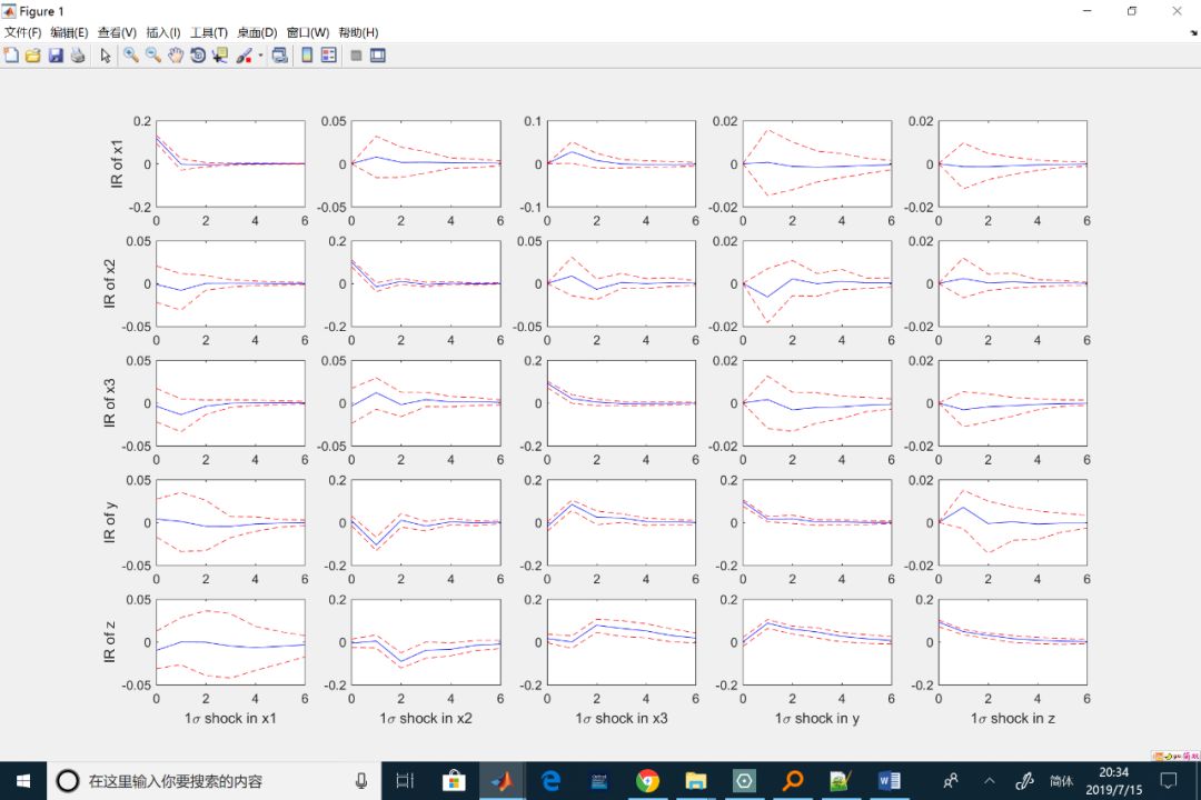
% impulse

[IRF, lb, ub] = irf3(result1,irfhmax, figureflag, irfalpha, bsnum, labels);

% variance decomposition

vd_mf = var_decomp(result1,vdhmax);

% causality test

disp('%%%%% Mixed Frequency, horizon = 1 %%%%%')

pval_mat1 =MFCTGK_all1(result1, m, K_H, gcbs, dispflag, gclabels);

disp('%%%%%%%%%%%%%%%%%%%%%%%%%%%%%%%%%%%%%%%%');

disp(blanks(3)');

%%%%%%%%%%%%%%%% REMARK%%%%%%%%%%%%%%%%%%%%%%%%%%%%%%%%%%%%%%%%%%%%%%%%%%%

% ... What can you tellfrom these results?

% Causality test says (1)x causes y, (2) y causes z, and there is no other causality.

%

% IRF verifies (1) and(2). IRF gives you one more important implication, though.

% It seems that x doeshave a significant impact on z! How is this ever possible?

%

% ... This is a typicalexample of "causal chain". x does cause z via y.

% To see this point, notethat:

%

% A^2 = [ 0.01,? -0.01,?0.06,??? 0,??? 0;

%??????? -0.01,??0.02,? 0.04,??? 0,???0;

%??????????? 0,????? 0,?0.01,??? 0,??? 0;

%??????? -0.09,?-0.09,? 0.09, 0.04,??? 0;

%??????????? 0,?-0.81,? 0.81, 0.72, 0.36]

%

% The lower-left block isno longer zeros.

% In bivariate casecausal chains are never possible, but in more general

% cases causal chains areof great importance.

% To capture causalityfrom x to z, we need to run two-step-ahead causality test.

%%%%%%%%%%%%%%%%%%%%%%%%%%%%%%%%%%%%%%%%%%%%%%%%%%%%%%%%%%%%%%%%%%%%%%%%%%%

result2 = VAR_est1(Data, p, 2,lambda);?

disp('%%%%% Mixed frequency, horizon = 2 %%%%%')

pval_mat2 =MFCTGK_all1(result2, m, K_H, gcbs, dispflag, gclabels);

disp('%%%%%%%%%%%%%%%%%%%%%%%%%%%%%%%%%%%%%%%%');

disp(blanks(3)');

% ... Now you can see xdoes cause z at horizon 2.

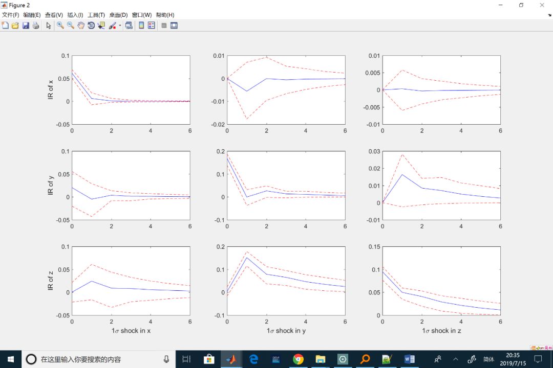
%% Step 3: Low frequencyanalysis

% for comparison,aggregate x into quarterly frequency (flow sampling)

Data_ = [mean(Data(:,1:3), 2),Data(:,4), Data(:,5)];

% fit VAR(1)

result_ = VAR_est1(Data_, p, 1,lambda);

% IRF

[IRF_, lb_, ub_] =irf3(result_, irfhmax, figureflag, irfalpha, bsnum, gclabels);

% variance decomposition

vd_lf = var_decomp(result_,vdhmax);

% causality test

disp('%%%%% Low Frequency, horizon = 1 %%%%%')

pval_mat_lf =CTGK_all1(result_, gcbs, dispflag, gclabels);

disp('%%%%%%%%%%%%%%%%%%%%%%%%%%%%%%%%%%%%%%%%');

%%%%%%%%%%%%%%%%%%%%%%REMARK %%%%%%%%%%%%%%%%%%%%%%%%%%%%%%%%%%%%%%%%%%%%%

% Based on low frequencymodel, you cannot observe x causing y.

% This is because thepositive impact of x3 on y and the negative impact of

% x2 on y offset eachother after flow aggregation.

% This highlights anadvantage of mixed frequency approach.

%%%%%%%%%%%%%%%%%%%%%%%%%%%%%%%%%%%%%%%%%%%%%%%%%%%%%%%%%%%%%%%%%%%%%%%%%%%

輸出結果

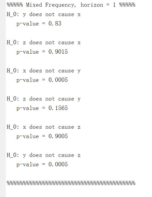
%%%%%Mixed Frequency, horizon = 1 %%%%%

H_0:y does not cause x

?? p-value = 0.83

H_0:z does not cause x

?? p-value = 0.9015

H_0:x does not cause y

?? p-value = 0.0005

H_0:z does not cause y

?? p-value = 0.1565

H_0:x does not cause z

?? p-value = 0.9005

H_0:y does not cause z

?? p-value = 0.0005

%%%%%%%%%%%%%%%%%%%%%%%%%%%%%%%%%%%%%%%%

%%%%%Mixed frequency, horizon = 2 %%%%%

H_0:y does not cause x

?? p-value = 0.0425

H_0:z does not cause x

?? p-value = 0.819

H_0:x does not cause y

?? p-value = 0.302

H_0:z does not cause y

?? p-value = 0.8695

H_0:x does not cause z

?? p-value = 0.0005

H_0:y does not cause z

?? p-value = 0.0005

%%%%%%%%%%%%%%%%%%%%%%%%%%%%%%%%%%%%%%%%

%%%%%Low Frequency, horizon = 1 %%%%%

H_0:y does not cause x

?? p-value = 0.275

H_0:z does not cause x

?? p-value = 0.924

H_0:x does not cause y

?? p-value = 0.789

H_0:z does not cause y

?? p-value = 0.029

H_0:x does not cause z

?? p-value = 0.5655

H_0:y does not cause z

?? p-value = 0.0005

%%%%%%%%%%%%%%%%%%%%%%%%%%%%%%%%%%%%%%%%

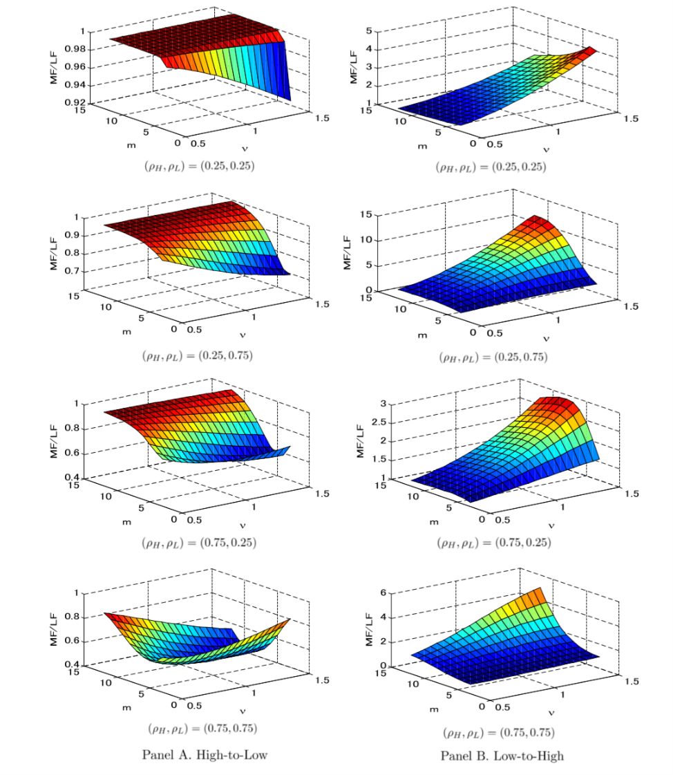
混合和低頻因果關系檢驗的局部漸近冪

MIDAS和NowCasting這塊的建模

本號后續發布，敬請關注

記得添加本號