Segmentaion標簽的三種表示：poly、mask、rle

不同于圖像分類這樣比較簡單直接的計算機視覺任務，圖像分割任務（又分為語義分割、實例分割、全景分割）的標簽形式稍為復雜。在分割任務中，我們需要在像素級上表達的是一張圖的哪些區域是哪個類別。

多邊形坐標Polygon

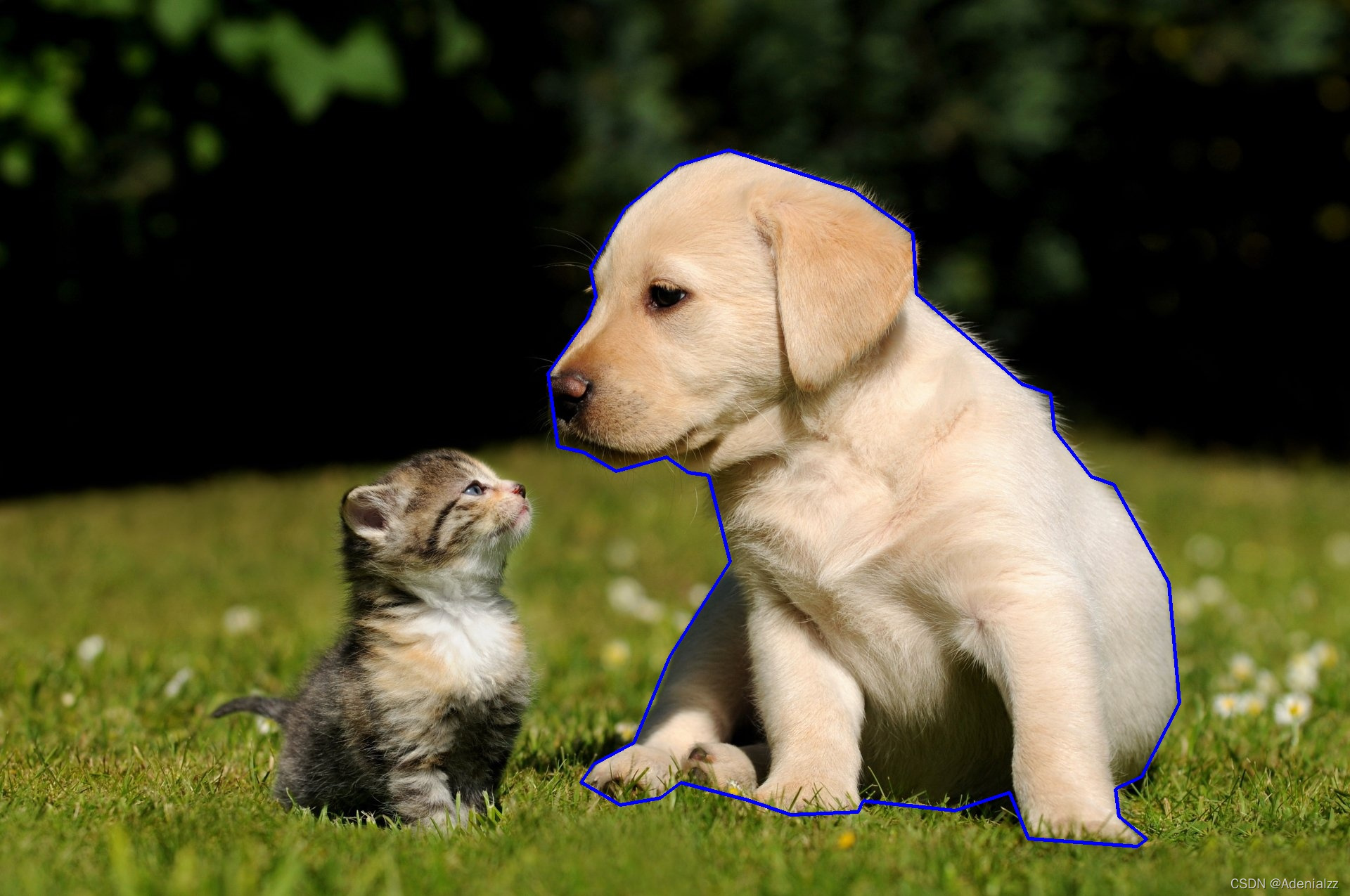
第一感下，要表達圖像中某個區域是什么類別，只要這個區域“圈起來”，并給它一個標簽就好了。的確，用多邊形來將目標圈出來確實是最符合我們視覺上對圖像的感知的方法。并且在很多數據集的標注過程中，來自人類的手工標注也是通過給出一個一個點的坐標，從而形成一個閉合的多邊形區域，從而實現對圖像中目標物體的分割。

我們通過 OpenCV 的 polylines 函數來將這種做法畫出來看一下：

import numpy as np
import cv2
cat_poly = [[390.56410256410254, 1134.179487179487], # ...[407.2307692307692, 1158.5384615384614]]dog_poly = [[794.4102564102564, 635.4615384615385], # ...[780.3076923076923, 531.6153846153846]]img = cv2.imread("cat-dog.jpeg")cat_points = np.array(cat_poly, dtype=np.int32)
cv2.polylines(img, [cat_points], True, (255, 0, 0), 3)
dog_points  = np.array(dog_poly, dtype=np.int32)
cv2.polylines(img, [dog_points], True, (0, 0, 255), 3)cv2.imshow("window", img)
cv2.waitKey(0)

這里的數據 cat_poly 是一個 $n×2n\times 2$ 的二維數組，表示多邊形框的 $n$ 個坐標，即 $x_1,y_1],[x_2,y_2],...[x_n,y_n]]$ 。畫出來大概就是下面這樣子：

在這里插入圖片描述

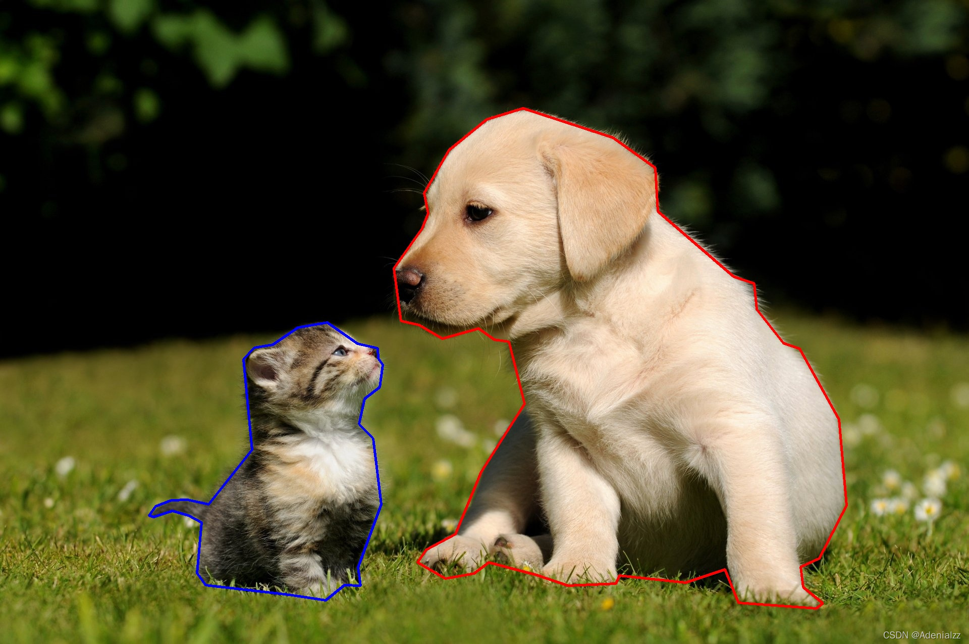
這樣的確可以劃分出我們想要的區域，但是沒有體現出“區域”的概念，即在整個多邊形框內，都是貓/狗區域。

掩膜區域Mask

為了體現出區域的概念，我們可以將整個區域展示出來，這里用到 fillPoly 函數，就是下面這樣大家常常見到的樣子：

img = cv2.imread("cat-dog.jpeg")dog_poly = [# ...
]
cat_poly = [# ...
]cat_points = np.array(cat_poly, dtype=np.int32)
dog_points = np.array(dog_poly, dtype=np.int32)zeros = np.zeros((img.shape), dtype=np.uint8)
mask = cv2.fillPoly(zeros, [cat_points], color=(255, 0, 0))
mask = cv2.fillPoly(zeros, [dog_points], color=(0, 0, 255))
mask_img = 0.5 * mask + imgcv2.imshow("window", mask_img)
cv2.waitKey(0)

在這里插入圖片描述

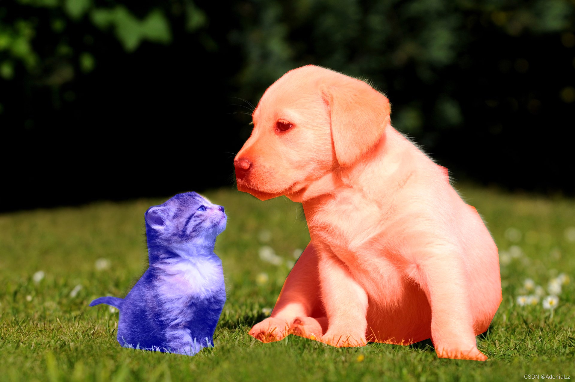
在模型的設計與訓練中，我們有時最后輸出的就是與原圖尺寸相同二值的 mask 圖，其中 1 的地方表示該位置有某一類物體，0 表示沒有該類物體。因此我們通常要將上面的多邊形標注轉為二值的 mask 圖來作為直接用來計算損失的標簽。由多邊形標簽轉為掩膜標簽的代碼如下：

def poly2mask(points, width, height):mask = np.zeros((width, height), dtype=np.int32)obj = np.array([points], dtype=np.int32)cv2.fillPoly(mask, obj, 1)return mask

這里的 points 就是上面我們的 cat_poly 這樣的二維數組的多邊形數據。

就是將有該類物體的地方置為1，其他為0，有些區別會在語義分割和實例分割中有所不同，可能是某一類有一個mask，也可能是每一個實例一個 mask。大家按需調整即可。

將上述貓狗的例子轉換后可視化如下：

width, height = img.shape[: 2]
cat_mask = poly2mask(cat_poly, width, height)
dog_mask = poly2mask(dog_poly, width, height)

注意，在做可視化時建議將上面的 poly2mask 函數中的 1 改為 255。因為灰度值為 1 也基本是黑的，但是在訓練中為 1 即可。

在這里插入圖片描述

從掩膜 mask 轉換回多邊形 poly 的函數會比較復雜，在這個過程中可能會有標簽精度的損失。我們用越多的坐標點來表示掩膜自然也就越精確，極端情況下，將掩膜邊緣處的每一個像素都連接起來，這時不會有精度的損失。但我們通常不會這樣做。

這里給出轉換的函數，該函數會返回一個數組，數組的長度就是 mask 中閉合區域的個數，數組的每個元素是一組坐標： $x_1,y_1,x_2,y_2,...,x_n,y_n]$ ，注意這里的坐標并不是成對的，與我們上面的數據輸入略有不同，因此在下面的實驗中，筆者用 get_paired_coord 函數統一了一下接口規范。

其中 tolerance 參數（中文意為容忍度）表示的就是輸出的多邊形的每個坐標點之間的最大距離，可想而知，該值越大，可能的精度損失越大。

from skimage import measuredef close_contour(contour):if not np.array_equal(contour[0], contour[-1]):contour = np.vstack((contour, contour[0]))return contourdef binary_mask_to_polygon(binary_mask, tolerance=0):"""Converts a binary mask to COCO polygon representationArgs:binary_mask: a 2D binary numpy array where '1's represent the objecttolerance: Maximum distance from original points of polygon to approximatedpolygonal chain. If tolerance is 0, the original coordinate array is returned."""polygons = []# pad mask to close contours of shapes which start and end at an edgepadded_binary_mask = np.pad(binary_mask, pad_width=1, mode='constant', constant_values=0)contours = measure.find_contours(padded_binary_mask, 0.5)contours = np.subtract(contours, 1)for contour in contours:contour = close_contour(contour)contour = measure.approximate_polygon(contour, tolerance)if len(contour) < 3:continuecontour = np.flip(contour, axis=1)segmentation = contour.ravel().tolist()# after padding and subtracting 1 we may get -0.5 points in our segmentationsegmentation = [0 if i < 0 else i for i in segmentation]polygons.append(segmentation)return polygons

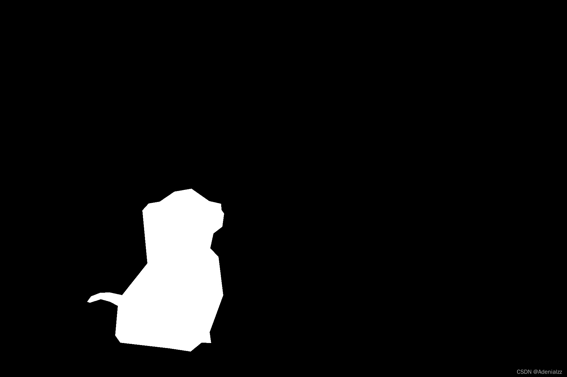
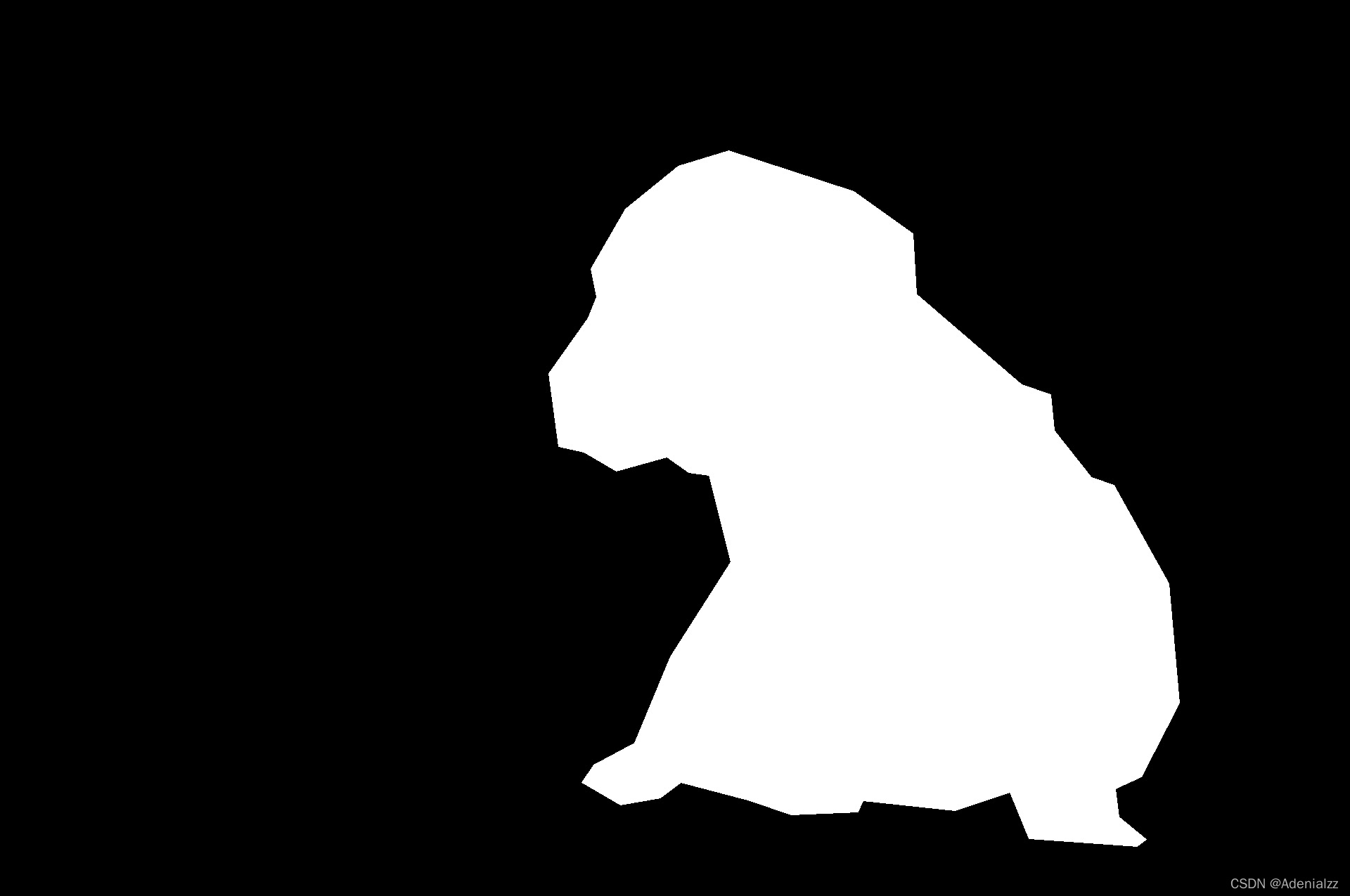
下面看一下本例中的小狗在 tolerance 為 0 和 100 下的區別。

def get_paired_coord(coord):points = Nonefor i in range(0, len(coord), 2):point = np.array(coord[i: i+2], dtype=np.int32).reshape(1, 2)if (points is None): points = pointelse: points = np.concatenate([points, point], axis=0)return pointspoly_0 = binary_mask_to_polygon(cat_mask+dog_mask, tolerance=0)
poly_100 = binary_mask_to_polygon(cat_mask+dog_mask, tolerance=100)poly0_0 = get_paired_coord(poly_0[0])		# poly_0[0]是小狗，poly[1]是小貓
poly100_0 = get_paired_coord(poly_100[0])p0_img = img
p0_points = np.array(poly0_0, dtype=np.int32)
cv2.polylines(p0_img, [p0_points], True, (255, 0, 0), 3)
cv2.imwrite("poly_dog_0.jpeg", p0_img)p100_img = cv2.imread("cat-dog.jpeg")
p100_points = np.array(poly100_0, dtype=np.int32)
cv2.polylines(p100_img, [p100_points], True, (255, 0, 0), 3)
cv2.imwrite("poly_dog_100.jpeg", p100_img)

在這里插入圖片描述

tolerance=0

在這里插入圖片描述

tolerance=100

與我們的預期相符，tolerance=0 時不會有精度損失，而當 tolerance=100 時可以看到進度損失已經比較大了。

RLE編碼

mask 大概是這種形式：

mask=np.array([[0, 0, 0, 0, 0, 0, 0, 0],[0, 0, 1, 1, 0, 0, 1, 0],[0, 0, 1, 1, 1, 1, 1, 0],[0, 0, 1, 1, 1, 1, 1, 0],[0, 0, 1, 1, 1, 1, 1, 0],[0, 0, 1, 0, 0, 0, 1, 0],[0, 0, 1, 0, 0, 0, 1, 0],[0, 0, 0, 0, 0, 0, 0, 0]])

可以看到其實是有很多信息冗余的，因為只有0，1兩種元素，RLE編碼就是將相同的數據進行壓縮計數，同時記錄當前數據出現的初始為位置和對應的長度，例如：[0,1,1,1,0,1,1,0,1,0] 編碼之后為1,3,5,2,8,1。其中的奇數位表示數字1出現的對應的index，而偶數位表示它對應的前面的坐標位開始數字1重復的個數。

RLE全稱（run-length encoding），翻譯為游程編碼，又譯行程長度編碼，又稱變動長度編碼法（run coding），在控制論中對于二值圖像而言是一種編碼方法，對連續的黑、白像素數(游程)以不同的碼字進行編碼。游程編碼是一種簡單的非破壞性資料壓縮法，其好處是加壓縮和解壓縮都非常快。其方法是計算連續出現的資料長度壓縮之。

RLE是COCO數據集的規范格式之一，也是許多圖像分割比賽指定提交結果的格式。

mask轉rle編碼，這里我們借助 pycocotools 工具包：

def singleMask2rle(mask):rle = mask_util.encode(np.array(mask[:, :, None], order='F', dtype="uint8"))[0]rle["counts"] = rle["counts"].decode("utf-8")return rle