項目原地址：

Hyperspectral-Classificationhttps://github.com/eecn/Hyperspectral-ClassificationDataLoader講解：

[高光譜]使用PyTorch的dataloader加載高光譜數據https://blog.csdn.net/weixin_37878740/article/details/130929358

一、模型加載

? ? ? ? 在原始項目中，提供了14種模型可供選擇，從最簡單的SVM到3D-CNN，這里以2D-CNN為例，在原項目中需要將model屬性設置為：sharma。

? ? ? ? ?模型通過一個get_model(.)函數獲得，該函數一共四個返回（model, optimizer, loss, hyperparams；分別為：模型，迭代器，損失函數，超參數），輸入為模型類別。

? ? ? ? 進入函數內部，找到對應的函數體如下：

elif name == 'sharma':kwargs.setdefault('batch_size', 60)        #batch_szieepoch = kwargs.setdefault('epoch', 30)     #迭代數lr = kwargs.setdefault('lr', 0.05)         #學習率center_pixel = True                        #是否開啟中心像素模型# We assume patch_size = 64kwargs.setdefault('patch_size', 64)        #patch_szie，即圖像塊大小model = SharmaEtAl(n_bands, n_classes, patch_size=kwargs['patch_size'])  #模型本體optimizer = optim.SGD(model.parameters(), lr=lr, weight_decay=0.0005)    #迭代器criterion = nn.CrossEntropyLoss(weight=kwargs['weights'])            #交叉熵損失函數kwargs.setdefault('scheduler', optim.lr_scheduler.MultiStepLR(optimizer, milestones=[epoch // 2, (5 * epoch) // 6], gamma=0.1))

? ? ? ? 這里設置了一部分超參數，同時設置了patch_size為64（此概念可以參見dataloader篇），采用的損失函數為常見的交叉熵損失函數，而模型本體則是使用SharmaEtAl(.)進行加載。

二、模型本體

? ? ? ? 跳轉至SharmaEtAl(nn.Module)，其繼承自nn.model，輸入參數3個，分別為：輸入通道數、分類數、圖塊尺寸。

def __init__(self, input_channels, n_classes, patch_size=64):

? 該網絡的結構如圖，模型中里面包含3個卷積、2個bn、2個池化和2個全連接，如下：

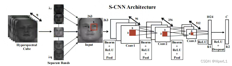
# 卷積層1
self.conv1 = nn.Conv3d(1, 96, (input_channels, 6, 6), stride=(1,2,2))
self.conv1_bn = nn.BatchNorm3d(96)
self.pool1 = nn.MaxPool3d((1, 2, 2))
# 卷積層2
self.conv2 = nn.Conv3d(1, 256, (96, 3, 3), stride=(1,2,2))
self.conv2_bn = nn.BatchNorm3d(256)
self.pool2 = nn.MaxPool3d((1, 2, 2))
# 卷積層3
self.conv3 = nn.Conv3d(1, 512, (256, 3, 3), stride=(1,1,1))# 展平函數
self.features_size = self._get_final_flattened_size()# 由兩個全連接組成的分類器
self.fc1 = nn.Linear(self.features_size, 1024)
self.dropout = nn.Dropout(p=0.5)
self.fc2 = nn.Linear(1024, n_classes)

? ? ? ? 其中的展平函數_get_final_flattened_size(.)，并不實際參與前向傳遞，僅計算轉換后的通道數。

    def _get_final_flattened_size(self):with torch.no_grad():x = torch.zeros((1, 1, self.input_channels,self.patch_size, self.patch_size))x = F.relu(self.conv1_bn(self.conv1(x)))x = self.pool1(x)print(x.size())b, t, c, w, h = x.size()x = x.view(b, 1, t*c, w, h) x = F.relu(self.conv2_bn(self.conv2(x)))x = self.pool2(x)print(x.size())b, t, c, w, h = x.size()x = x.view(b, 1, t*c, w, h) x = F.relu(self.conv3(x))print(x.size())_, t, c, w, h = x.size()return t * c * w * h

? ? ? ? 實際的前向傳遞如下：

    def forward(self, x):# 卷積塊1x = F.relu(self.conv1_bn(self.conv1(x)))x = self.pool1(x)# 獲取tensor尺寸b, t, c, w, h = x.size()# 調整tensor尺寸x = x.view(b, 1, t*c, w, h) # 卷積塊2x = F.relu(self.conv2_bn(self.conv2(x)))x = self.pool2(x)# 獲取tensor尺寸b, t, c, w, h = x.size()# 調整tensor尺寸x = x.view(b, 1, t*c, w, h) # 卷積塊3x = F.relu(self.conv3(x))# 調整tensor尺寸x = x.view(-1, self.features_size)# 分類器x = self.fc1(x)x = self.dropout(x)x = self.fc2(x)return x

三、訓練與測試

? ? ? ? 主函數中，訓練和測試結構如下：

        try:train(model, optimizer, loss, train_loader, hyperparams['epoch'],scheduler=hyperparams['scheduler'], device=hyperparams['device'],supervision=hyperparams['supervision'], val_loader=val_loader,display=viz)except KeyboardInterrupt:# Allow the user to stop the trainingpassprobabilities = test(model, img, hyperparams)prediction = np.argmax(probabilities, axis=-1)

? ? ? ? 訓練被封裝在train(.)函數中，測試封裝在test(.)函數中，下面逐一來看。

? ? ? ? 首先是train函數，這里省去外圍部分，僅看核心的循環控制段。

# 外循環控制，用于控制輪次(epoch)
for e in tqdm(range(1, epoch + 1), desc="Training the network"):# 進入訓練模式net.train()avg_loss = 0.# 從dataloader中取出圖像(data)和標簽(target)for batch_idx, (data, target) in tqdm(enumerate(data_loader), total=len(data_loader)):# 如果是GPU模式則需要轉換為cuda格式data, target = data.to(device), target.to(device)#---實際的訓練部分---## 凍結梯度optimizer.zero_grad()# 訓練模式（監督訓練/半監督訓練）if supervision == 'full':# 前向傳遞output = net(data)#target = target - 1# 交叉熵損失函數loss = criterion(output, target)elif supervision == 'semi':outs = net(data)output, rec = outs#target = target - 1loss = criterion[0](output, target) + net.aux_loss_weight * criterion[1](rec, data)#---實際的訓練部分---## 損失函數反向傳遞loss.backward()# 迭代器步進optimizer.step()# 記錄損失函數avg_loss += loss.item()losses[iter_] = loss.item()mean_losses[iter_] = np.mean(losses[max(0, iter_ - 100):iter_ + 1])iter_ += 1del(data, target, loss, output)

? ? ? ? 接下來是test函數，與train不同的是，其參數為：model, img, hyperparams。其中img，是一整張高光譜圖像，而不是由DataSet塊采樣后的圖像塊。故其結構也與train大不相同。

? ? ? ? 在進行測試的時候，需要一個滑動窗口(sliding_window)函數將其進行切塊以滿足圖像輸入的要求。同時還需要一個grouper函數將其組裝為batch送入神經網絡中。所以我們可以看到循環控制的最外層實際上就是上面兩個函數來組成的。

    # 圖像切塊iterations = count_sliding_window(img, **kwargs) // batch_sizefor batch in tqdm(grouper(batch_size, sliding_window(img, **kwargs)),total=(iterations),desc="Inference on the image"):#  鎖定梯度with torch.no_grad():#  逐像素模式if patch_size == 1:data = [b[0][0, 0] for b in batch]data = np.copy(data)data = torch.from_numpy(data)# 其他模式else:data = [b[0] for b in batch]data = np.copy(data)data = data.transpose(0, 3, 1, 2)data = torch.from_numpy(data)data = data.unsqueeze(1)indices = [b[1:] for b in batch]# 類型轉換data = data.to(device)# 前向傳遞output = net(data)if isinstance(output, tuple):output = output[0]output = output.to('cpu')if patch_size == 1 or center_pixel:output = output.numpy()else:output = np.transpose(output.numpy(), (0, 2, 3, 1))for (x, y, w, h), out in zip(indices, output):# 將得到的像素平裝回原尺寸if center_pixel:probs[x + w // 2, y + h // 2] += outelse:probs[x:x + w, y:y + h] += outreturn probs

? ? ? ? 這個函數會使用上述的兩個函數，將圖像切割成可以放入神經網絡的尺寸并逐個進行前向傳遞，最后將得到的所有像素的結果按照原來的尺寸組成一個結果矩陣返回。

? ? ? ? 最后，這個結果由一個argmax函數得到其概率最大的預測結果：

prediction = np.argmax(probabilities, axis=-1)

四、結果計算

? ? ? ? 在完成上述步驟后，由metrics(.)函數計算最終的模型結果：

run_results = metrics(prediction, test_gt, ignored_labels=hyperparams['ignored_labels'], n_classes=N_CLASSES)

? ? ? ? 其函數體如下：

def metrics(prediction, target, ignored_labels=[], n_classes=None):"""Compute and print metrics (accuracy, confusion matrix and F1 scores).Args:prediction: list of predicted labelstarget: list of target labelsignored_labels (optional): list of labels to ignore, e.g. 0 for undefn_classes (optional): number of classes, max(target) by defaultReturns:accuracy, F1 score by class, confusion matrix"""ignored_mask = np.zeros(target.shape[:2], dtype=np.bool)for l in ignored_labels:ignored_mask[target == l] = Trueignored_mask = ~ignored_mask#target = target[ignored_mask] -1target = target[ignored_mask]prediction = prediction[ignored_mask]results = {}n_classes = np.max(target) + 1 if n_classes is None else n_classescm = confusion_matrix(target,prediction,labels=range(n_classes))results["Confusion matrix"] = cm# Compute global accuracytotal = np.sum(cm)accuracy = sum([cm[x][x] for x in range(len(cm))])accuracy *= 100 / float(total)results["Accuracy"] = accuracy# Compute F1 scoreF1scores = np.zeros(len(cm))for i in range(len(cm)):try:F1 = 2. * cm[i, i] / (np.sum(cm[i, :]) + np.sum(cm[:, i]))except ZeroDivisionError:F1 = 0.F1scores[i] = F1results["F1 scores"] = F1scores# Compute kappa coefficientpa = np.trace(cm) / float(total)pe = np.sum(np.sum(cm, axis=0) * np.sum(cm, axis=1)) / \float(total * total)kappa = (pa - pe) / (1 - pe)results["Kappa"] = kappareturn results