介紹 (Introduction)

I am going to show you the different ways you can build a football league table in Excel. Some of the methods are old school but others utilise Excel’s new capabilities.

我將向您展示在Excel中建立足球聯賽表格的不同方法。 其中一些方法過時，而另一些則利用Excel的新功能。

In case you weren’t already aware, Excel has undergone a big change to its calculation engine fairly recently. The concept of dynamic arrays was first introduced back in September 2018, however, for many Microsoft 365 users the first batch of new functions took an awfully long time to appear. Unless you have been an Office Insider, you will not have been able to use them. Even though the update was rolled out to my copy towards the start of the year, there were still swathes of users who were kept waiting.

如果您還沒有意識到，Excel會在最近對其計算引擎進行重大更改。 動態數組的概念最早是在2018年9月引入的，但是，對于許多Microsoft 365用戶而言，第一批新功能花了很長時間才出現。 除非您是Office Insider，否則您將無法使用它們。 即使更新已于今年年初發布到我的副本中，但仍有大量用戶一直在等待。

Since dynamic arrays were introduced in Excel, array formulas no long require you to press Ctrl + Shift + Return every time you edit a cell. This was an annoying practice that made many users, including myself, reluctant to use arrays. They just didn’t feel like a native and integrated part of Excel. Now you can use an array formula like any other — without that additional step.

由于動態數組是在Excel中引入的，因此數組公式不再需要您每次編輯單元格時都按Ctrl + Shift + Return。 這種令人討厭的做法使許多用戶(包括我自己)都不愿意使用數組。 他們只是感覺不像Excel的本地集成部分。 現在，您可以像其他數組一樣使用數組公式了-無需執行其他步驟。

If you want to find out more about the new functions, I recommend you visit Microsoft’s help page for each one: XLOOKUP, FILTER, UNIQUE, SORTBY, SORT, SEQUENCE, RANDARRAY.

如果您想了解有關新功能的更多信息，建議您訪問Microsoft的每個幫助頁面： XLOOKUP ， FILTER ， UNIQUE ， SORTBY ， SORT ， SEQUENCE ， RANDARRAY 。

開始之前 (Before we start)

Download the workbook from here: https://bit.ly/39mlqkp.

從此處下載工作簿： https : //bit.ly/39mlqkp 。

Quick caveat: if you have an older version of Excel, you will find some of the examples do not work because of compatibility issues. This is unavoidable unless you purchase a Microsoft 365 subscription. Personally, I would recommend you do so.

快速警告：如果您使用的是舊版Excel，則會發現某些示例由于兼容性問題而無法使用。 除非您購買Microsoft 365訂閱，否則這是不可避免的。 就個人而言，我建議您這樣做。

采取的步驟 (Steps taken)

Firstly, a dataset is required containing a list of all the matches played and their respective results. I have used English Premier League data from the 2019/20 season for this example. To conserve space elsewhere, the matches are stored in a separate worksheet called Data — with the table itself named DataTable.

首先，需要一個數據集，其中包含所有進行的比賽及其各自結果的列表。 在此示例中，我使用了2019/20賽季的英超聯賽數據。 為了節省其他地方的空間，匹配項存儲在名為Data的單獨工作表中，表本身名為DataTable 。

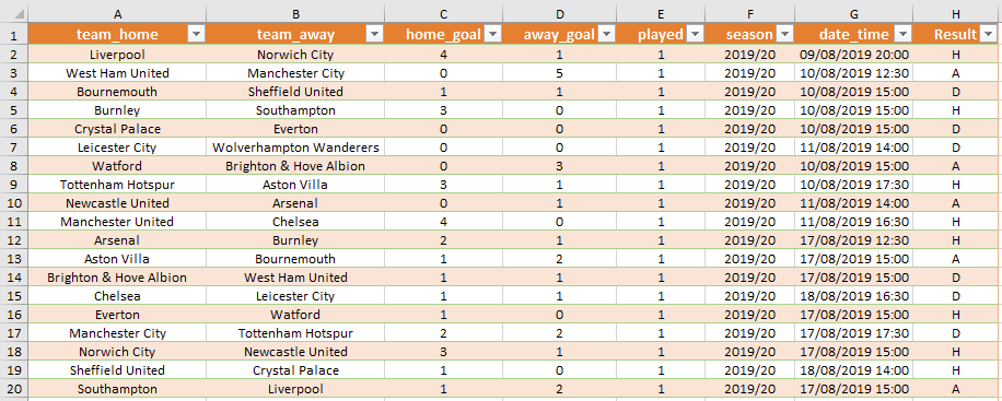
You’ll notice there’s a calculated column on the end called Result. This formula looks at the home_goal and away_goal fields for each match played and determines whether the outcome was a home win (H), draw (D) or away win (A).

您會注意到最后有一個計算列Result 。 該公式查看每場比賽的home_goal和away_goal字段，并確定結果是主場獲勝( H )，平局( D )還是客場獲勝( A )。

There are three sections: Part A, Part B and Part C. Each contains multiple league tables that output identical values, but the method used differs.

共有三個部分： A 部分，B 部分和C部分 。 每個表都包含多個輸出相同值的聯賽表，但是使用的方法不同。

Any kind of system that involves ranking data is typically going to require an unordered and ordered table. The former houses the mathematical calculations and determines the ranking of each row, whilst the latter references it to output the data in the correct order. Part A and Part B are based off this principle. Part C, however, contains two variants that are not dependent on an additional table.

任何涉及對數據進行排名的系統通常都需要無序和有序的表。 前者存儲數學計算并確定每行的排名，而后者引用它以按正確的順序輸出數據。 A部分和B部分基于此原理。 但是， C部分包含兩個不依賴于其他表的變體。

The tables in the workbook use these headers:

工作簿中的表使用以下標頭：

• POS (position)

  POS ( 位置 )

• TEAM

  球隊

• P (matches played)

  P (參加比賽)

• W (matches won)

  W (贏得比賽)

• D (matches drawn)

  D (匹配結果)

• L (matches lost)

  L (輸掉比賽)

• F (goals for)

  F (目標)

• A (goals against)

  A (反對)

• GD (goal difference)

  GD (目標差)

• PTS (points)

  PTS (點)

• RANK* (table position when points are sorted in descending order)

  RANK *( 點按降序排序時的表位置 )

*Table A2 only

*僅限表A2

甲部 (Part A)

The approaches here are all based on official Excel tables. The way to tell if what looks like a table is indeed a table— is to check if it has a small blue triangle in the bottom-right, or to click on it and the Table Design tab will appear in the ribbon.

這里的方法都是基于官方的Excel表。 判斷表看起來是否確實是表的方法是 ：檢查表的右下角是否有一個小的藍色三角形，或者單擊它，然后“表設計”選項卡將出現在功能區中。

We start off by creating Table A1, which is unordered and forms the base for Table A2, Table A3 and Table A4 to work off. The P, W, D, L columns use COUNTIFS formulas to count the number of matches a team has played, won, drawn and lost respectively. It’s important to note that a single COUNTIFS formula only allows for AND conditions. That means all criteria must be met for a successful count. As we have home and away matches to consider, we need to use two COUNTIFS statements in the same cell to add the counts together. The same concept applies to the SUMIFS function, which has been used for the columns that involve addition: F and A.

我們首先創建表A1，它是無序的，并構成了表A2，表A3和表A4的基礎 。 P ， W ， D ， L列使用COUNTIFS公式來計算球隊分別打過，贏過，輸過和輸過的比賽次數。 重要的是要注意，單個COUNTIFS公式僅允許AND條件。 這意味著必須滿足所有條件才能成功計數。 考慮到本場比賽和客場比賽，我們需要在同一單元格中使用兩個COUNTIFS語句將計數加在一起。 相同的概念適用于SUMIFS函數，該函數已用于涉及加法的列： F和A。

The goal difference (GD) column is as simple as F minus A. Custom formatting has also been applied so positive numbers are preceded by a ‘+’ symbol and negatives with a ‘-’.

目標差( GD )列很簡單，即F減去A。 自定義格式也已應用，因此正數前帶有“ +”符號，負數前帶有“-”。

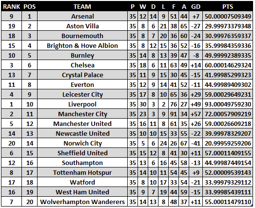
The PTS column uses a rather convoluted formula to produce a very long number, but is necessary so the ordered table sorts correctly. In the case of tiebreakers, where two or more teams are level on points, we need to ensure a unique ranking for each team. The priority order that determines rank is as follows:

PTS列使用一個相當復雜的公式來產生一個很長的數字，但是這是必需的，因此有序表可以正確排序。 對于平局決勝局，其中兩個或更多團隊在得分上持平，我們需要確保每個團隊的排名都是唯一的。 確定等級的優先級順序如下：

1. Points (PTS)

1.點數( PTS )

2. Goal difference (GD)

2.目標差( GD )

3. Goals scored (F)

3.進球( F )

4. First letter of Team name (TEAM)

4.團隊名稱的首字母( TEAM )

5. Position number (POS)

5.職位編號( POS )

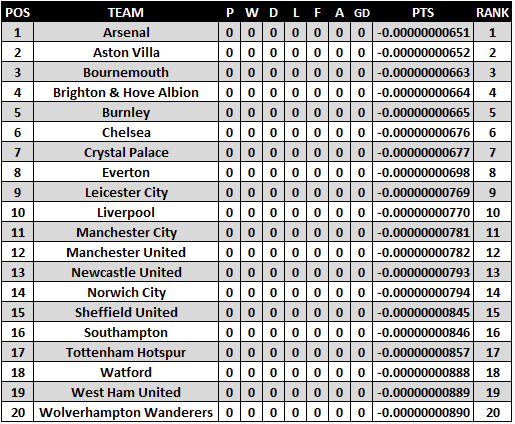
To prove the points column works, we set the values of the P/W/D/L/F/A/GD/PTS columns to pure zeros. With all things being level now, the numbers in RANK directly mirror the alphabetical order of the teams. If you look at Arsenal and Aston Villa, for example, both of them begin with the letter ‘A’, so the only thing separating their points are the position numbers.

為了證明points列有效，我們將P / W / D / L / F / A / GD / PTS列的值設置為純零。 現在一切都平了， RANK中的數字直接反映了球隊的字母順序。 例如，如果您查看阿森納(Arsenal)和阿斯頓維拉(Aston Villa)，它們都以字母'A'開頭，因此，將它們分開的唯一點就是位置編號。

Table A2 uses VLOOKUP to extract the relevant data from Table A1 and display it in the correctly sorted order. VLOOKUP is a popular function, but is less flexible than INDEX/MATCH and the new XLOOKUP. For this reason, many people will stop using it once they’ve discovered one of the latter two.

表A2使用VLOOKUP從表A1中提取相關數據并以正確排序的順序顯示它們。 VLOOKUP是一種流行的功能，但不如INDEX / MATCH和新的XLOOKUP靈活。 因此，一旦發現后兩者之一，許多人就會停止使用它。

One of the biggest downsides of VLOOKUP is having to reorder your data so that the lookup range is the furthest-left column. In this case, the RANK column has had to be moved in Table A1 so it comes before all the columns that we want to return data from.

VLOOKUP的最大缺點之一是必須對數據重新排序，以使查找范圍在最左列。 在這種情況下，必須在表A1中移動RANK列，因此它位于我們要從中返回數據的所有列之前。

This is not the case with INDEX/MATCH and XLOOKUP. It doesn’t matter about the position of the RANK column. With both Table A3 and Table A4, we have simply referenced only the ranges we need from Table A1.

INDEX / MATCH和XLOOKUP并非如此。 RANK列的位置無關緊要。 對于表A3和表A4 ，我們僅引用了表A1中需要的范圍。

B部分 (Part B)

Unlike Part A, all three of the ‘tables’ you see are not actually tables—in Excel terms anyway—although we’ll still use that term. Table B1 uses only 11 formulas—one for the headings and the other 10 for the calculations. To surprise you even more: Table B2 and Table B3 use just three. This is what dynamic arrays are all about. They grow and shrink depending on the output of the formula. This concept goes completely against traditional Excel, where one cell has one formula. The big advantage of this is you are less likely to make errors in your worksheet and will reduce inconsistencies.

與A部分不同，您看到的所有三個“表”實際上都不是表(無論如何以Excel術語而言)，盡管我們仍將使用該術語。 表B1僅使用11個公式-一個用于標題，另一個10個用于計算。 更讓您驚訝的是： 表B2和表B3僅使用三個。 這就是動態數組的全部意義。 它們根據公式的輸出而增長和收縮。 此概念完全與傳統的Excel相抵觸，在Excel中，一個單元格只有一個公式。 這樣做的最大好處是，您不太可能在工作表中出錯，并且可以減少不一致的情況。

For the column headings of each table, we have used an array constant to hold the column names. These are fixed values and do not change. Unfortunately, only numbers and text strings can be used in constants — not formulas.

對于每個表的列標題，我們使用了一個數組常量來保存列名。 這些是固定值，不會改變。 不幸的是，常量中只能使用數字和文本字符串，而不能用于公式。

={"POS","TEAM","P","W","D","L","F","A","GD","PTS"}

You will notice in the formulas that a cell reference followed by a hashtag is a common occurrence. This is a spilled range, meaning it is dynamic, so its size will adapt according to the data.

您會在公式中注意到，單元格引用后跟井號是常見的情況。 這是一個溢出范圍，意味著它是動態的，因此其大小將根據數據進行調整。

We have again used COUNTIFS and SUMIFS for the P/W/D/L/F/A columns in the same manner as we did in Table A1, except spilled ranges have replaced regular ones.

我們再次以與表A1中相同的方式對P / W / D / L / F / A列使用COUNTIFS和SUMIFS，只是溢出范圍已替換常規范圍。

Some of the new Excel functions have been utilised and allow us to do a lot from a single cell.

一些新的Excel函數已被利用，使我們可以在單個單元格中完成很多工作。

For the POS column, the SEQUENCE function returns a set of numbers. By wrapping it around the COUNTA function, it will always return an incremental number in accordance to how many teams are displayed adjacent to it.

對于POS列，SEQUENCE函數返回一組數字。 通過將它包裝在COUNTA函數周圍，它將始終根據與其相鄰顯示的團隊數量返回一個遞增的數字。

POS: =SEQUENCE(COUNTA(D14#))

POS： =SEQUENCE(COUNTA(D14#))

The individual team names have been extracted from the team_home column in DataTable using UNIQUE, and then sorted in ascending order using SORT.

已使用UNIQUE從DataTable的team_home列中提取了各個團隊名稱，然后使用SORT以升序對其進行了排序。

TEAM: =SORT(UNIQUE(DataTable[team_home]))

團隊： =SORT(UNIQUE(DataTable[team_home]))

Notice how the PTS column is full of integers and there is no RANK column. This is because we no longer need that awfully complex calculation you saw in Table A1. What replaces it then? The trusty SORT function again.

請注意， PTS列是如何充滿整數，而沒有RANK列。 這是因為我們不再需要您在表A1中看到的非常復雜的計算。 那有什么替代呢？ 可信賴的SORT功能再次發揮作用。

You’ll see in Table B2 and Table B3 that the formula for the table calculations starts at the very top of TEAM. That’s one formula controlling 180 values!

您將在表B2和表B3中看到表計算公式從TEAM的最頂部開始。 這是一個控制180個值的公式！

CHOOSE and SWITCH are great for this purpose. Multiple column values can be stored in one formula and spill vertically and horizontally.

選擇和切換非常適合此目的。 多個列值可以存儲在一個公式中，并且可以垂直和水平溢出。

Let’s look at the main formula in Table B2:

讓我們看一下表B2中的主要公式：

=SORT(CHOOSE({1,2,3,4,5,6,7,8,9},
D14#,
E14#,
F14#,
G14#,
H14#,
I14#,
J14#,
K14#,
L14#
),{9,8,6,1},-1,-1,-1,1)

The numbers at the top between the parentheses are placed in the index_num argument. They are the index numbers that refer to each spilled range below it.

括號之間頂部的數字放在index_num參數中。 它們是引用其下方每個溢出范圍的索引號。

The {9,8,6,1} in the sort_index argument refers to the sorting order and the {-1,-1,-1,1} in sort_order determines whether each sort_index number should be sorted ascending or descending.

sort_index參數中的{9,8,6,1}指的是排序順序， sort_order的{-1,-1,-1,1}確定每個sort_index編號應升序還是降序。

Just like in Table A1, we have a priority list: PTS, GD, F and TEAM. But it’s so much easier to implement it this new way though.

就像表A1一樣 ，我們有一個優先級列表： PTS ， GD ， F和TEAM 。 但是，以這種新方式實現它要容易得多。

The SWITCH method shown in Table C3 is very similar to the CHOOSE one, but the advantage is you are not limited to index numbers, so you can name values what you wish. This is ideal if you have a long formula and you want to optimise readability.

表C3中顯示的SWITCH方法與CHOOSE方法非常相似，但是優點是您不僅限于索引號，因此可以根據需要命名值。 如果您有一個較長的公式并且想要優化可讀性，那么這是理想的選擇。

=SORT(SWITCH({"Team","P","W","D","L","F","A","GD","PTS"},
"Team",
D14#,
"P",
E14#,
"W",
F14#,
"D",
G14#,
"L",
H14#,
"F",
I14#,
"A",
J14#,
"GD",
K14#,
"PTS",
L14#
),{9,8,6,1},{-1,-1,-1,1})

C部分 (Part C)

The first thing you’ll probably notice in this section is that there is no unordered table. The two table variants you see are both self-contained, and only depend on the dataset in the Data worksheet. We have simply squeezed in all the formulas you saw in Table B1 and placed them in a CHOOSE (Table C1) and SWITCH (Table C2) statement.

在本節中您可能會注意到的第一件事是沒有無序表。 您看到的兩個表變體都是獨立的，并且僅取決于數據工作表中的數據集。 我們只是簡單地擠壓了在表B1中看到的所有公式，并將它們放在CHOOSE( 表C1 )和SWITCH( 表C2 )語句中。

These really are the true definition of a ‘mega formula’! They are rather overwhelming to look at, but using line breaks appropriately (Alt + Return) to spread out the formula can solve most of the readability issues. I also recommend using the SWITCH option as named values can allow you to immediately see where each section starts and ends.

這些確實是“超級公式”的真實定義！ 他們看上去不知所措，但是適當地使用換行符(Alt + Return)來展開公式可以解決大多數可讀性問題。 我還建議使用SWITCH選項，因為命名值可以使您立即看到每個部分的開始和結束位置。

One of the limitations of Excel formulas is the inability to reuse parts of a formula. For example, with the goal difference column, rather than having to repeat the formulas for columns F and A, it’d be nice if it was possible to access those values and reuse them for a different part of the formula. Given the LET function is closer upon us, this may well solve that problem for the most part, as we’ll be able to declare variables at the start of a formula and use them multiple times within the same formula.

Excel公式的局限性之一是無法重用公式的某些部分。 例如，使用目標差列，而不必重復列F和A的公式，那么可以訪問這些值并將它們重新用于公式的其他部分，那就太好了。 鑒于LET函數離我們越來越近，這可以在很大程度上解決該問題，因為我們將能夠在公式的開頭聲明變量，并在同一公式中多次使用它們。

最后的話 (Final Words)

Please see the workbook for all the examples. Hopefully they will give you food for thought for how you can go about creating formulas that make use of Excel’s dynamic array powers. The centralised, one formula = many cells approach will gradually become the de facto standard, so get ahead of the curve whilst you can.

請參閱工作簿中的所有示例。 希望他們能為您提供思考，幫助您如何使用Excel的動態數組功能創建公式。 集中的，一個公式=許多單元的方法將逐漸成為事實上的標準，因此盡您所能，走在曲線前。

Workbook download: https://bit.ly/39mlqkp.

工作簿下載： https : //bit.ly/39mlqkp 。

學習功能 (Functions to learn)

There are many resources on the web that enable you to learn in-depth about the functions used in the workbook. I’ve found Exceljet to be a particularly helpful source.

Web上有許多資源，使您可以深入了解工作簿中使用的功能。 我發現Exceljet是特別有用的資源。

RANK.EQ

排名

COUNTIFS

COUNTIFS

SUMIFS

SUMIFS

VLOOKUP

VLOOKUP

INDEX

指數

MATCH

比賽

COUNTA

COUNTA

CHOOSE

選擇

SWITCH

開關

COLUMN

柱

CODE

碼

UNIQUE

獨特

SORT

分類

XLOOKUP

XLOOKUP

SEQUENCE

序列