Note from Towards Data Science’s editors: While we allow independent authors to publish articles in accordance with our rules and guidelines, we do not endorse each author’s contribution. You should not rely on an author’s works without seeking professional advice. See our Reader Terms for details.

Towards Data Science編輯的注意事項： 盡管我們允許獨立作者按照我們的 規則和指南 發表文章 ，但我們不認可每位作者的貢獻。 您不應在未征求專業意見的情況下依賴作者的作品。 有關 詳細信息， 請參見我們的 閱讀器條款 。

算法交易策略開發 (Algorithmic Trading Strategy Development)

Backtesting is the hallmark of quantitative trading. Backtesting takes historical or synthetic market data and tests the profitability of algorithmic trading strategies. This topic demands expertise in statistics, computer science, mathematics, finance, and economics. This is exactly why in large quantitative trading firms there are specific roles for individuals with immense knowledge (usually at the doctorate level) of the respective subjects. The necessity for expertise cannot be understated as it separates winning (or seemingly winning) trading strategies from losers. My goal for this article is to break up what I consider an elementary backtesting process into a few different sections…

回測是定量交易的標志。 回測采用歷史或合成市場數據，并測試算法交易策略的盈利能力。 本主題需要統計，計算機科學，數學，金融和經濟學方面的專業知識。 這就是為什么在大型定量交易公司中，對于具有相應學科的豐富知識(通常是博士學位)的個人，要發揮特定的作用。 專業知識的必要性不可低估，因為它將成功(或看似成功)的交易策略與失敗者分開。 本文的目的是將我認為是基本的回測過程分為幾個不同的部分……

• I. The Backtesting Engine

  I.回測引擎

• II. Historical and Synthetic Data Management

  二。 歷史和綜合數據管理

• III. Backtesting Metrics

  三， 回測指標

• IV. Live Implementation

  IV。 現場實施

• V. Pitfalls in Strategy Development

  五 ，戰略發展中的陷阱

回測引擎 (The Backtesting Engine)

The main backtesting engine will be built in Python using a library called backtrader. Backtrader makes it incredibly easy to build trading strategies and implement them on historical data immediately. The entire library centers around the Cerebro class. As the name implies, you can think of this as the brain or engine of the backtest.

主要的回測引擎將使用稱為backtrader的庫在Python中構建 。 Backtrader使得建立交易策略并立即在歷史數據上實施交易變得異常容易。 整個圖書館圍繞著Cerebro類。 顧名思義，您可以將其視為回測的大腦或引擎。

import backtrader as btdef backtesting_engine(symbol, strategy, fromdate, todate, args=None):"""Primary function for backtesting, not entirely parameterized"""# Backtesting Enginecerebro = bt.Cerebro()

I decided to build a function so I can parameterize different aspects of the backtest on the fly (and eventually build a pipeline). The next backtrader class we need to discuss is the Strategy class. If you look at the function I built to house the instance of Cerebro you’ll see that it takes a strategy as an input — this is expecting a backtrader Strategy class or subclass. Subclasses of the Strategy class are exactly what we will be using to build our own strategies. If you need a polymorphism & inheritance refresher or don’t know what that means see my article 3 Python Concepts in under 3 minutes. Let’s build a strategy for our backtest…

我決定構建一個函數，以便可以動態地對回測的不同方面進行參數化(并最終構建管道)。 我們需要討論的下一個回購者類是策略類。 如果您查看我為容納Cerebro實例而構建的功能，您會看到它以策略作為輸入-這是期待的回購商Strategy類或子類。 策略類的子類正是我們用來構建自己的策略的類。 如果您需要多態和繼承復習器，或者不知道這意味著什么，請在3分鐘之內閱讀我的文章3 Python概念 。 讓我們為回測制定策略...

from models.isolation_model import IsolationModel
import backtrader as bt
import pandas as pd
import numpy as npclass MainStrategy(bt.Strategy):'''Explanation:MainStrategy houses the actions to take as a stream of data flows in a linear fashion with respect to time'''def log(self, txt, dt=None):''' Logging function fot this strategy'''dt = dt or self.datas[0].datetime.date(0)print('%s, %s' % (dt.isoformat(), txt))def __init__(self, data):# Keep a reference to the "close" line in the data[0] dataseriesself.dataopen = self.datas[0].openself.datahigh = self.datas[0].highself.datalow = self.datas[0].lowself.dataclose = self.datas[0].closeself.datavolume = self.datas[0].volume

In the MainStrategy, Strategy subclass above I create fields that we are interested in knowing about before making a trading decision. Assuming a daily data frequency the fields we have access to every step in time during the backstep are…

在上面的MainStrategy，Strategy子類中，我創建了我們感興趣的字段，這些字段是我們在做出交易決策之前要了解的。 假設每天的數據頻率，在后退步驟中我們可以訪問的每個時間段的字段是……

• Day price open
  當日價格開盤
• Day price close
  當天收盤價
• Day price low
  當日價格低
• Day price high
  當天價格高
• Day volume
  日成交量

It doesn’t take a genius to understand that you cannot use the high, low, and close to make an initial or intraday trading decision as we don’t have access to that information in realtime. However, it is useful if you want to store it and access that information from previous days.

理解您不能使用高，低和接近來做出初始或盤中交易決策并不需要天才，因為我們無法實時訪問該信息。 但是，如果您要存儲它并訪問前幾天的信息，這將很有用。

The big question in your head right now should be where is the data coming from?

您現在腦海中最大的問題應該是數據來自哪里？

The answer to that question is in the structure of the backtrader library. Before we run the function housing Cerebro we will add all the strategies we want to backtest, and a data feed — the rest is all taken care of as the Strategy superclass holds the datas series housing all the market data.

該問題的答案在于backtrader庫的結構。 在運行帶有Cerebro的功能之前，我們將添加我們要回測的所有策略以及一個數據提要-其余所有工作都將得到處理，因為Strategy超類擁有容納所有市場數據的數據系列。

This makes our lives extremely easy.

這使我們的生活變得極為輕松。

Let’s finish the MainStrategy class by making a simple long-only mean reversion style trading strategy. To access a tick of data we override the next function and add trading logic…

讓我們通過制定一個簡單的長期均值回歸樣式交易策略來結束MainStrategy類。 要訪問數據變動，我們將覆蓋下一個功能并添加交易邏輯…

from models.isolation_model import IsolationModel
import backtrader as bt
import pandas as pd
import numpy as npclass MainStrategy(bt.Strategy):'''Explanation:MainStrategy houses the actions to take as a stream of data flows in a linear fashion with respect to time
'''def log(self, txt, dt=None):''' Logging function fot this strategy'''dt = dt or self.datas[0].datetime.date(0)print('%s, %s' % (dt.isoformat(), txt))def __init__(self):self.dataclose = self.datas[0].closeself.mean = bt.indicators.SMA(period=20)self.std = bt.indicators.StandardDeviation()self.orderPosition = 0self.z_score = 0def next(self):self.log(self.dataclose[0])z_score = (self.dataclose[0] - self.mean[0])/self.std[0]if (z_score >= 2) & (self.orderPosition > 0):self.sell(size=1)if z_score <= -2:self.log('BUY CREATE, %.2f' % self.dataclose[0])self.buy(size=1)self.orderPosition += 1

Every day gets a z-score calculated for it (number of standard deviations from the mean) based on its magnitude we will buy or sell equity. Please note, yes I am using the day’s close to make the decision, but I’m also using the day’s close as an entry price to my trade — it would be wiser to use the next days open.

每天都會根據其大小來計算z得分(相對于平均值的標準偏差的數量)，我們將買賣股票。 請注意，是的，我使用當天的收盤價來做決定，但是我也將當天的收盤價用作我交易的入場價-使用第二天的開盤價會更明智。

The next step is to add the strategy to our function housing the Cerebro instance…

下一步是將策略添加到容納Cerebro實例的功能中…

import backtrader as bt
import pyfolio as pfdef backtesting_engine(symbol, strategy, fromdate, todate, args=None):"""Primary function for backtesting, not entirely parameterized"""# Backtesting Enginecerebro = bt.Cerebro()# Add a Strategy if no Data Required for the modelif args is None:cerebro.addstrategy(strategy)# If the Strategy requires a Model and therefore dataelif args is not None:cerebro.addstrategy(strategy, args)

In the code above I add the strategy provided to the function to the Cerebro instance. This is beyond the scope of the article but I felt pressed to include it. If the strategy that we are backtesting requires additional data (some AI model) we can provide it in the args parameter and add it to the Strategy subclass.

在上面的代碼中，我將為函數提供的策略添加到Cerebro實例。 這超出了本文的范圍，但是我迫切希望將其包括在內。 如果要回測的策略需要其他數據(某些AI模型)，則可以在args參數中提供它，并將其添加到Strategy子類中。

Next, we need to find a source of historical or synthetic data.

接下來，我們需要找到歷史或綜合數據的來源。

歷史和綜合數據管理 (Historical and Synthetic Data Management)

I use historical and synthetic market data synonymously as some researchers have found synthetic data indistinguishable (and therefore is more abundant as its generative) from other market data. For the purposes of this example we will be using the YahooFinance data feed provided by backtrader, again making implementation incredibly easy…

我將歷史和綜合市場數據作為同義詞使用，因為一些研究人員發現綜合數據與其他市場數據是無法區分的(因此，其生成量更大)。 出于本示例的目的，我們將使用backtrader提供的YahooFinance數據供稿，再次使實現變得異常容易。

import backtrader as bt
import pyfolio as pfdef backtesting_engine(symbol, strategy, fromdate, todate, args=None):"""Primary function for backtesting, not entirely parameterized"""# Backtesting Enginecerebro = bt.Cerebro()# Add a Strategy if no Data Required for the modelif args is None:cerebro.addstrategy(strategy)# If the Strategy requires a Model and therefore dataelif args is not None:cerebro.addstrategy(strategy, args)# Retrieve Data from YahooFinancedata = bt.feeds.YahooFinanceData(dataname=symbol,fromdate=fromdate,  # datetime.date(2015, 1, 1)todate=todate,  # datetime.datetime(2016, 1, 1)reverse=False)# Add Data to Backtesting Enginecerebro.adddata(data)

It’s almost ridiculous how easy it is to add a data feed to our backtest. The data object uses backtraders YahooFinanceData class to retrieve data based on the symbol, fromdate, and todate. Afterwards, we simply add that data to the Cerebro instance. The true beauty in backtrader’s architecture comes in realizing that the data is automatically placed within, and iterated through every strategy added to the Cerebro instance.

將數據提要添加到我們的回測中是多么容易，這簡直太荒謬了。 數據對象使用backtraders YahooFinanceData類根據符號，起始日期和起始日期檢索數據。 然后，我們只需將該數據添加到Cerebro實例中即可。 backtrader架構的真正美在于實現將數據自動放入其中，并通過添加到Cerebro實例的每種策略進行迭代。

回測指標 (Backtesting Metrics)

There are a variety of metrics used to evaluate the performance of a trading strategy, we’ll cover a few in this section. Again, backtrader makes it extremely easy to add analyzers or performance metrics. First, let’s set an initial cash value for our Cerebro instance…

有多種指標可用于評估交易策略的績效，本節將介紹其中的一些指標。 同樣，backtrader使添加分析器或性能指標變得非常容易。 首先，讓我們為Cerebro實例設置初始現金價值...

import backtrader as bt
import pyfolio as pfdef backtesting_engine(symbol, strategy, fromdate, todate, args=None):"""Primary function for backtesting, not entirely parameterized"""# Backtesting Enginecerebro = bt.Cerebro()# Add a Strategy if no Data Required for the modelif args is None:cerebro.addstrategy(strategy)# If the Strategy requires a Model and therefore dataelif args is not None:cerebro.addstrategy(strategy, args)# Retrieve Data from YahooFinancedata = bt.feeds.YahooFinanceData(dataname=symbol,fromdate=fromdate,  # datetime.date(2015, 1, 1)todate=todate,  # datetime.datetime(2016, 1, 1)reverse=False)# Add Data to Backtesting Enginecerebro.adddata(data)# Set Initial Portfolio Valuecerebro.broker.setcash(100000.0)

There are a variety of metrics we can use to evaluate risk, return, and performance — let’s look at a few of them…

我們可以使用多種指標來評估風險，回報和績效-讓我們看看其中的一些…

夏普比率 (Sharpe Ratio)

As referenced in the show Billions, the amount of return per unit of risk, the Sharpe Ratio. Defined as follows…

如顯示的“十億”所示，單位風險的收益金額即夏普比率。 定義如下...

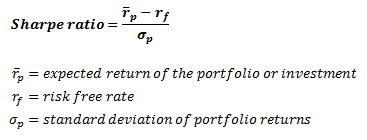
Several downfalls, and assumptions. It’s based on historical performance, assumes normal distributions, and can often be used to incorrectly compare portfolios. However, it’s still a staple to any strategy or portfolio.

幾次失敗和假設。 它基于歷史表現，假定為正態分布，并且經常被用來錯誤地比較投資組合。 但是，它仍然是任何策略或投資組合的主要內容。

System Quality Number

系統質量編號

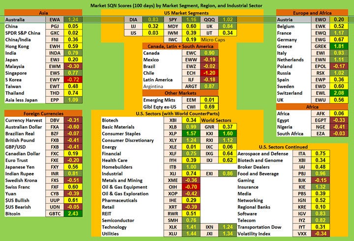
An interesting metric I’ve always enjoyed using as it includes volume of transactions in a given period. Computed by multiplying the SQN by the number of trades and dividing the product by 100. Below is a chart of values across different segments, regions, and sectors.

我一直喜歡使用的有趣指標，因為它包含給定時間段內的交易量。 通過將SQN乘以交易數量并將乘積除以100進行計算。以下是不同細分市場，區域和部門的價值圖表。

Let’s now add these metrics to Cerebro and run the backtest…

現在讓我們將這些指標添加到Cerebro并進行回測...

import backtrader as bt
import pyfolio as pfdef backtesting_engine(symbol, strategy, fromdate, todate, args=None):"""Primary function for backtesting, not entirely parameterized"""# Backtesting Enginecerebro = bt.Cerebro()# Add a Strategy if no Data Required for the modelif args is None:cerebro.addstrategy(strategy)# If the Strategy requires a Model and therefore dataelif args is not None:cerebro.addstrategy(strategy, args)# Retrieve Data from Alpacadata = bt.feeds.YahooFinanceData(dataname=symbol,fromdate=fromdate,  # datetime.date(2015, 1, 1)todate=todate,  # datetime.datetime(2016, 1, 1)reverse=False)# Add Data to Backtesting Enginecerebro.adddata(data)# Set Initial Portfolio Valuecerebro.broker.setcash(100000.0)# Add Analysis Toolscerebro.addanalyzer(bt.analyzers.SharpeRatio, _name='sharpe')# Of course we want returns too ;Pcerebro.addanalyzer(bt.analyzers.Returns, _name='returns')cerebro.addanalyzer(bt.analyzers.SQN, _name='sqn')# Starting Portfolio Valueprint('Starting Portfolio Value: %.2f' % cerebro.broker.getvalue())# Run the Backtesting Enginebacktest = cerebro.run()# Print Analysis and Final Portfolio Valueprint('Final Portfolio Value: %.2f' % cerebro.broker.getvalue())print('Return: ', backtest[0].analyzers.returns.get_analysis())print('Sharpe Ratio: ', backtest[0].analyzers.sharpe.get_analysis())print('System Quality Number: ', backtest[0].analyzers.sqn.get_analysis())

Now, all we have to do is run the code above and we get the performance of our strategy based on the metrics we specified…

現在，我們要做的就是運行上面的代碼，并根據指定的指標獲得策略的性能……

from datetime import datetime
from strategies.reversion_strategy import LongOnlyReversion
from tools.backtesting_tools import backtesting_engine"""Script for backtesting strategies
"""if __name__ == '__main__':# Run backtesting enginebacktesting_engine(symbol='AAPL', strategy=LongOnlyReversion,fromdate=datetime(2018, 1, 1), todate=datetime(2019, 1, 1))

Here is the output…

這是輸出...

Starting Portfolio Value: 100000.002018-01-30, 160.95
2018-01-30, BUY CREATE, 160.952018-01-31, 161.4
2018-02-01, 161.74
2018-02-02, 154.72
2018-02-02, BUY CREATE, 154.72
2018-02-05, 150.85
2018-02-05, BUY CREATE, 150.85
2018-02-06, 157.16
2018-02-07, 153.792018-02-08, 149.56
2018-02-09, 151.39
2018-02-12, 157.49
2018-02-13, 159.07
2018-02-14, 162.0
2018-02-15, 167.44
2018-02-16, 166.9
2018-02-20, 166.332018-02-21, 165.58
2018-02-22, 166.96
2018-02-23, 169.87
2018-02-26, 173.23
2018-02-27, 172.66
2018-02-28, 172.42018-03-01, 169.38
2018-03-02, 170.55
2018-03-05, 171.15
2018-03-06, 171.0
2018-03-07, 169.41
2018-03-08, 171.26
2018-03-09, 174.2
2018-03-12, 175.89
2018-03-13, 174.19
2018-03-14, 172.71
2018-03-15, 172.92
2018-03-16, 172.31
2018-03-19, 169.67
2018-03-20, 169.62
2018-03-21, 165.77
2018-03-21, BUY CREATE, 165.77
2018-03-22, 163.43
2018-03-22, BUY CREATE, 163.43
2018-03-23, 159.65
2018-03-23, BUY CREATE, 159.652018-03-26, 167.22
2018-03-27, 162.94
2018-03-28, 161.14
2018-03-29, 162.4
2018-04-02, 161.33
2018-04-03, 162.99
2018-04-04, 166.1
2018-04-05, 167.252018-04-06, 162.98
2018-04-09, 164.59
2018-04-10, 167.69
2018-04-11, 166.91
2018-04-12, 168.55
2018-04-13, 169.12
2018-04-16, 170.18
2018-04-17, 172.522018-04-18, 172.13
2018-04-19, 167.25
2018-04-20, 160.4
2018-04-23, 159.94
2018-04-24, 157.71
2018-04-25, 158.4
2018-04-26, 158.952018-04-27, 157.11
2018-04-30, 159.96
2018-05-01, 163.67
2018-05-02, 170.9
2018-05-03, 171.212018-05-04, 177.93
2018-05-07, 179.22
2018-05-08, 180.08
2018-05-09, 181.352018-05-10, 183.94
2018-05-11, 183.24
2018-05-14, 182.81
2018-05-15, 181.15
2018-05-16, 182.842018-05-17, 181.69
2018-05-18, 181.03
2018-05-21, 182.31
2018-05-22, 181.85
2018-05-23, 183.02
2018-05-24, 182.812018-05-25, 183.23
2018-05-29, 182.57
2018-05-30, 182.18
2018-05-31, 181.57
2018-06-01, 184.84
2018-06-04, 186.392018-06-05, 187.83
2018-06-06, 188.482018-06-07, 187.97
2018-06-08, 186.26
2018-06-11, 185.812018-06-12, 186.83
2018-06-13, 185.29
2018-06-14, 185.39
2018-06-15, 183.48
2018-06-18, 183.392018-06-19, 180.42
2018-06-20, 181.21
2018-06-21, 180.2
2018-06-22, 179.68
2018-06-25, 177.0
2018-06-25, BUY CREATE, 177.002018-06-26, 179.2
2018-06-27, 178.94
2018-06-28, 180.24
2018-06-29, 179.862018-07-02, 181.87
2018-07-03, 178.7
2018-07-05, 180.14
2018-07-06, 182.64
2018-07-09, 185.172018-07-10, 184.95
2018-07-11, 182.55
2018-07-12, 185.61
2018-07-13, 185.9
2018-07-16, 185.5
2018-07-17, 186.022018-07-18, 185.0
2018-07-19, 186.44
2018-07-20, 186.01
2018-07-23, 186.18
2018-07-24, 187.53
2018-07-25, 189.292018-07-26, 188.7
2018-07-27, 185.56
2018-07-30, 184.52
2018-07-31, 184.89
2018-08-01, 195.78
2018-08-02, 201.51
2018-08-03, 202.09
2018-08-06, 203.14
2018-08-07, 201.24
2018-08-08, 201.37
2018-08-09, 202.96
2018-08-10, 202.35
2018-08-13, 203.66
2018-08-14, 204.52
2018-08-15, 204.99
2018-08-16, 208.0
2018-08-17, 212.15
2018-08-20, 210.08
2018-08-21, 209.67
2018-08-22, 209.682018-08-23, 210.11
2018-08-24, 210.77
2018-08-27, 212.5
2018-08-28, 214.22
2018-08-29, 217.42
2018-08-30, 219.41
2018-08-31, 221.952018-09-04, 222.66
2018-09-05, 221.21
2018-09-06, 217.53
2018-09-07, 215.78
2018-09-10, 212.882018-09-11, 218.26
2018-09-12, 215.55
2018-09-13, 220.76
2018-09-14, 218.25
2018-09-17, 212.44
2018-09-18, 212.79
2018-09-19, 212.92
2018-09-20, 214.542018-09-21, 212.23
2018-09-24, 215.28
2018-09-25, 216.65
2018-09-26, 214.92
2018-09-27, 219.34
2018-09-28, 220.112018-10-01, 221.59
2018-10-02, 223.56
2018-10-03, 226.282018-10-04, 222.3
2018-10-05, 218.69
2018-10-08, 218.19
2018-10-09, 221.212018-10-10, 210.96
2018-10-11, 209.1
2018-10-12, 216.57
2018-10-15, 211.94
2018-10-16, 216.612018-10-17, 215.67
2018-10-18, 210.63
2018-10-19, 213.84
2018-10-22, 215.14
2018-10-23, 217.172018-10-24, 209.72
2018-10-25, 214.31
2018-10-26, 210.9
2018-10-29, 206.94
2018-10-30, 207.98
2018-10-31, 213.42018-11-01, 216.67
2018-11-02, 202.3
2018-11-02, BUY CREATE, 202.30
2018-11-05, 196.56
2018-11-05, BUY CREATE, 196.562018-11-06, 198.68
2018-11-06, BUY CREATE, 198.68
2018-11-07, 204.71
2018-11-08, 204.02018-11-09, 200.06
2018-11-12, 189.99
2018-11-12, BUY CREATE, 189.99
2018-11-13, 188.09
2018-11-13, BUY CREATE, 188.092018-11-14, 182.77
2018-11-14, BUY CREATE, 182.77
2018-11-15, 187.28
2018-11-16, 189.362018-11-19, 181.85
2018-11-20, 173.17
2018-11-20, BUY CREATE, 173.17
2018-11-21, 172.972018-11-23, 168.58
2018-11-26, 170.86
2018-11-27, 170.48
2018-11-28, 177.042018-11-29, 175.68
2018-11-30, 174.73
2018-12-03, 180.84
2018-12-04, 172.88
2018-12-06, 170.952018-12-07, 164.86
2018-12-10, 165.94
2018-12-11, 165.0
2018-12-12, 165.46
2018-12-13, 167.27
2018-12-14, 161.91
2018-12-17, 160.41
2018-12-18, 162.49
2018-12-19, 157.42
2018-12-20, 153.45
2018-12-20, BUY CREATE, 153.45
2018-12-21, 147.48
2018-12-21, BUY CREATE, 147.48
2018-12-24, 143.67
2018-12-24, BUY CREATE, 143.67
2018-12-26, 153.78
2018-12-27, 152.78
2018-12-28, 152.86
2018-12-31, 154.34
Final Portfolio Value: 100381.48
Return:  OrderedDict([('rtot', 0.0038075421029081335), ('ravg', 1.5169490449833201e-05), ('rnorm', 0.003830027474518453), ('rnorm100', 0.3830027474518453)])
Sharpe Ratio:  OrderedDict([('sharperatio', None)])
System Quality Number:  AutoOrderedDict([('sqn', 345.9089929588268), ('trades', 2)])

現場實施 (Live Implementation)

This is less of a section more of a collection of resources that I have for implementing trading strategies. If you want to move forward and implement your strategy in a live market check out these articles…

這不是本節的更多內容，更多的是我用于實施交易策略的資源集合。 如果您想繼續前進并在實時市場中實施策略，請查看以下文章…

• Algorithmic Trading with Python

  使用Python進行算法交易

• Build an AI Stock Trading Bot for Free

  免費建立AI股票交易機器人

• Algorithmic Trading System Development

  算法交易系統開發

• Multithreading in Python for Finance

  Python for Finance中的多線程

• How to Build a Profitable Stock Trading Bot

  如何建立一個有利可圖的股票交易機器人

• Build a Neural Network to Manage a Stock Portfolio

  建立一個神經網絡來管理股票投資組合

算法交易策略的陷阱 (Algorithmic Trading Strategy Pitfalls)

• Not understanding the drivers of profitability in a strategy: There are some that believe, regardless of the financial or economic drivers, if you can get enough data and stir it up in such a way that you can develop a profitable trading strategy. I did too when I was younger, newer to the algorithmic trading, and more naive. The truth is if you can’t understand the nature of your own trading algorithmic it will never be profitable.

  不了解策略中獲利能力的驅動因素：有人認為，無論財務或經濟驅動因素如何，如果您能夠獲取足夠的數據并以一種可以制定有利可圖的交易策略的方式進行攪動，便會認為這是可行的。 當我還年輕，算法交易較新且天真時，我也這樣做了。 事實是，如果您不了解自己的交易算法的性質，它將永遠不會盈利。

• Not understanding how to split historical or synthetic data to both search for and optimize strategies: This one is big and the consequences are dire. I had a colleague back in college tell me he developed a system with a 300% return trading energy. Naturally, and immediately, I knew he completely overfitted a model to historical data and never actually implemented it in live data. Asking a simple question about his optimization process confirmed my suspicion.

  不了解如何拆分歷史數據或合成數據以同時搜索和優化策略 ：這一步很大，后果非常嚴重。 我上大學時曾有一位同事告訴我，他開發了一種具有300％的收益交易能量的系統。 自然而又立即地，我知道他完全將模型擬合到歷史數據中，而從未真正在實時數據中實現它。 問一個關于他的優化過程的簡單問題證實了我的懷疑。

• Not willing to accept down days: This one is interesting, and seems to have a greater effect on newer traders more than experienced ones. The veterans know there will be down days, losses, but the overarching goal is to have (significantly) more wins than losses. This issue generally arises in deployment — assuming that the other processes

  不愿接受低迷的日子：這很有趣，而且似乎對新手的影響要大于經驗豐富的人。 退伍軍人知道會有損失的日子，但是總的目標是勝利(多于失敗)。 通常在部署過程中會出現此問題-假設其他過程

• Not willing to retire a formerly profitable system: Loss control, please understand risk-management and loss control. Your system was successful, and that’s fantastic — that means you understand the design process and can do it again. Don’t get caught up in how well it did look at how well it’s doing. This has overlap with understanding the drivers of profitability in your strategy — you will know when and why it’s time to retire a system if you understand why it’s no longer profitable.

  不愿意淘汰以前有利可圖的系統：損失控制，請了解風險管理和損失控制。 您的系統成功了，這太棒了-這意味著您了解設計過程并可以再次執行。 不要被它的表現看得如何。 這與了解戰略中獲利的驅動因素有很多重疊-如果您了解為什么不再有利潤，您將知道何時以及為何該退休系統。