機器學習 (Machine Learning)

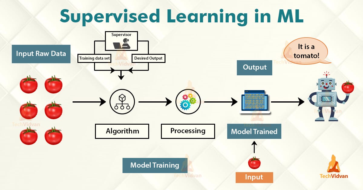
Machine learning is an application of artificial intelligence that provides systems the ability to automatically learn and improve from experience without being explicitly programmed. The 3 main categories of machine learning are supervised learning, unsupervised learning, and reinforcement learning. In this post, we shall focus on supervised learning for classification problems.

中號 achine學習是人工智能，它提供系統能夠自動學習并從經驗中提高，而不明確地編程能力的應用。 機器學習的3個主要類別是監督學習，無監督學習和強化學習。 在這篇文章中，我們將專注于分類問題的監督學習。

Supervised learning learns from past data and applies the learning to present data to predict future events. In the context of classification problems, the input data is labeled or tagged as the right answer to enable accurate predictions.

監督學習從過去的數據中學習，并將學習應用于當前的數據以預測未來的事件。 在分類問題的上下文中，將輸入數據標記或標記為正確答案，以實現準確的預測。

Tree-based learning algorithms are one of the most commonly used supervised learning methods. They empower predictive models with high accuracy, stability, ease of interpretation, and are adaptable at solving any classification or regression problem.

基于樹的學習算法是最常用的監督學習方法之一。 它們使預測模型具有較高的準確性，穩定性，易解釋性，并且適用于解決任何分類或回歸問題。

Decision Tree predicts the values of responses by learning decision rules derived from features. In a tree structure for classification, the root node represents the entire population, while decision nodes represent the particular point where the decision tree decides on which specific feature to split on. The purity for each feature will be assessed before and after the split. The decision tree will then decide to split on a specific feature that produces the purest leaf nodes (ie. terminal nodes at each branch).

決策樹通過學習從要素派生的決策規則來預測響應的值。 在用于分類的樹結構中 ， 根節點代表整個種群，而決策節點則代表決策樹確定要分割的特定特征的特定點。 在拆分之前和之后，將評估每個功能部件的純度。 然后，決策樹將決定拆分產生一個最純葉節點 (即每個分支的終端節點)的特定功能。

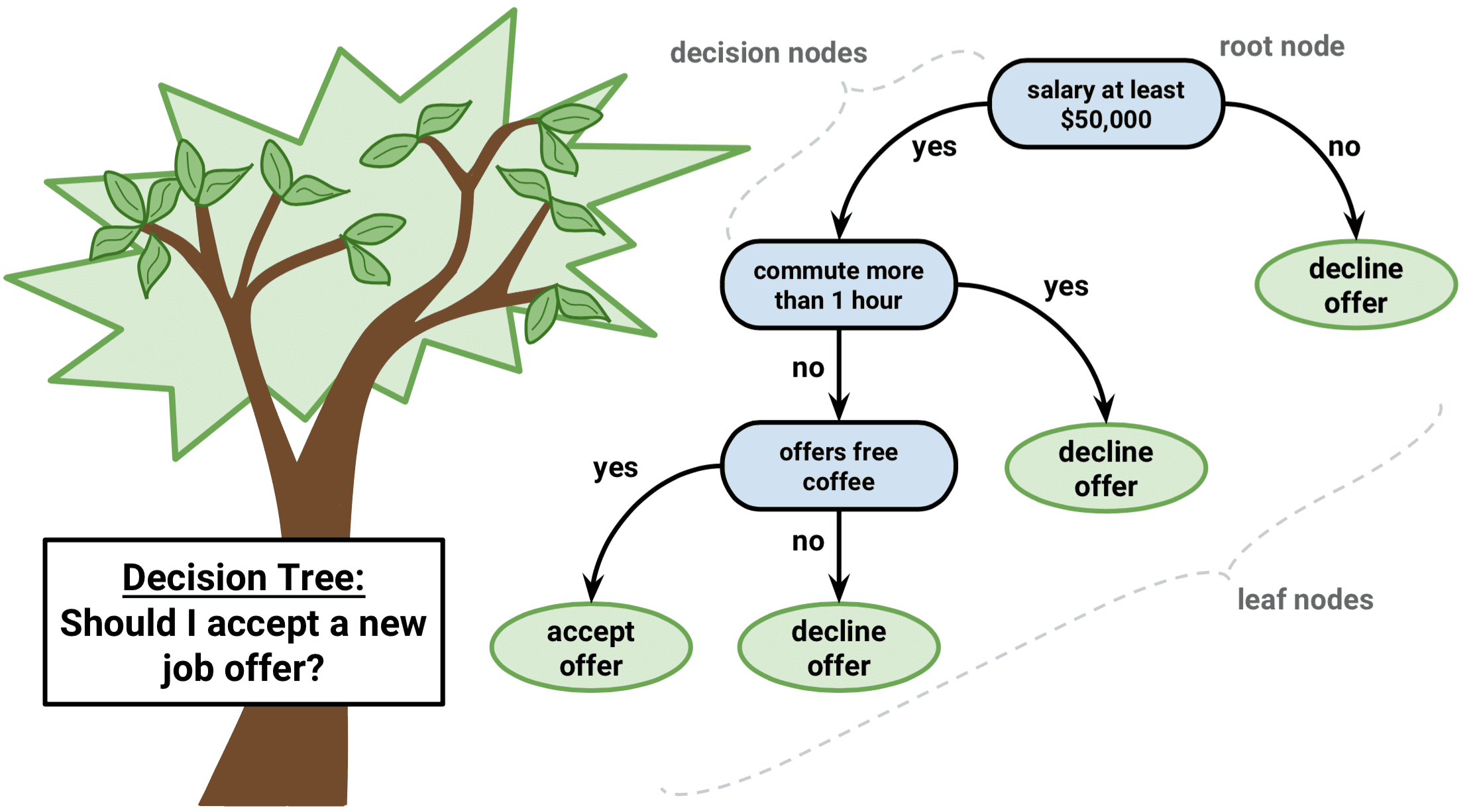
A significant advantage of a decision tree is that it forces the consideration of all possible outcomes of a decision and traces each path to a conclusion. It creates a comprehensive analysis of the consequences along each branch and identifies decision nodes that need further analysis.

決策樹的顯著優勢在于，它可以強制考慮決策的所有可能結果，并跟蹤得出結論的每條路徑。 它對每個分支的后果進行全面分析，并確定需要進一步分析的決策節點。

However, a decision tree has its own limitations. The reproducibility of the decision tree model is highly sensitive, as a small change in the data can result in a large change in the tree structure. Space and time complexity of the decision tree model is relatively higher, leading to longer model training time. A single decision tree is often a weak learner, hence a bunch of decision tree (known as random forest) is required for better prediction.

但是， 決策樹有其自身的局限性 。 決策樹模型的可重復性非常敏感，因為數據的微小變化會導致樹形結構的巨大變化。 決策樹模型的時空復雜度相對較高，導致模型訓練時間更長。 單個決策樹通常學習能力較弱，因此需要一堆決策樹(稱為隨機森林)才能更好地進行預測。

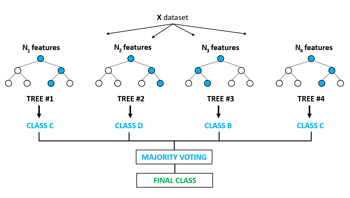
The random forest is a more powerful model that takes the idea of a single decision tree and creates an ensemble model out of hundreds or thousands of trees to reduce the variance. Thus giving the advantage of obtaining a more accurate and stable prediction.

隨機森林是一個功能更強大的模型，它采用單個決策樹的概念，并從數百或數千棵樹中創建一個集成模型以減少差異。 因此具有獲得更準確和穩定的預測的優勢 。

Each tree is trained on a random set of observations, and for each split of a node, only a random subset of the features is used for making a split. When making predictions, the random forest does not suffer from overfitting as it averages the predictions for each of the individual decision trees, for each data point, in order to arrive at a final classification.

每棵樹都在一組隨機的觀測值上訓練，并且對于節點的每個拆分，僅使用特征的隨機子集進行拆分。 在進行預測時，隨機森林不會遭受過度擬合的影響，因為它會針對每個數據點對每個單獨決策樹的預測取平均，以得出最終分類。

We shall approach a classification problem and explore the basics of how decision trees work, how individual decisions trees are combined to form a random forest, how to fine-tune the hyper-parameters to optimize random forest, and ultimately discover the strengths of using random forests.

我們將研究分類問題，并探索決策樹如何工作，如何將單個決策樹組合以形成隨機森林，如何微調超參數以優化隨機森林的基礎知識，并最終發現使用隨機森林的優勢。森林。

問題陳述：預測一個人每年的收入是否超過50,000美元。 (Problem Statement: To predict whether a person makes more than U$50,000 per year.)

讓我們開始編碼！ (Let’s start coding!)

import pandas as pd
import numpy as np
from sklearn.preprocessing import LabelEncoder
from sklearn.feature_selection import SelectKBest
from sklearn.feature_selection import chi2
from sklearn.utils import resample
from sklearn.model_selection import train_test_split
from sklearn import preprocessing
from sklearn.tree import DecisionTreeClassifier
from sklearn.tree import plot_tree
from sklearn.ensemble import RandomForestClassifier
from sklearn.model_selection import GridSearchCV
from sklearn import metrics
from sklearn.metrics import accuracy_score, precision_score, recall_score, f1_score
from sklearn.metrics import classification_report, precision_recall_curve, roc_curve, roc_auc_score
import scikitplot as skplt
import matplotlib.pyplot as plt
import seaborn as sns
%matplotlib inline

資料準備 (Data Preparation)

Load the Census Income Dataset from the URL and display the top 5 rows to inspect the data.

從URL加載人口普查收入數據集 ，并顯示前5行以檢查數據。

# Add header=None as the first row of the file contains the names of the columns. 
# Add engine='python' to avoid parser warning raised for reading a file that doesn’t use the default ‘c’ parser.income_data = pd.read_csv('https://archive.ics.uci.edu/ml/machine-learning-databases/adult/adult.data', header=None, delimiter=', ', engine='python')
income_data.head()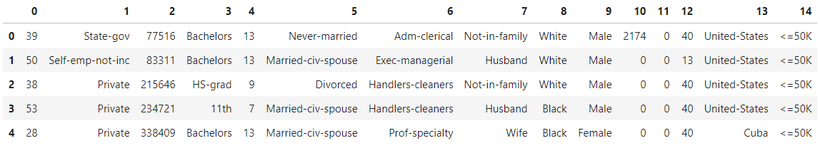

# Add headers to dataset
headers = ['age','workclass','fnlwgt','education','education_num','marital_status','occupation','relationship','race','sex','capital_gain','capital_loss','hours_per_week','native_country','income']income_data.columns = headers
income_data.head()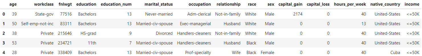

數據清理 (Data Cleaning)

# Check for empty cells and if data types are correct for the respective columns
income_data.info()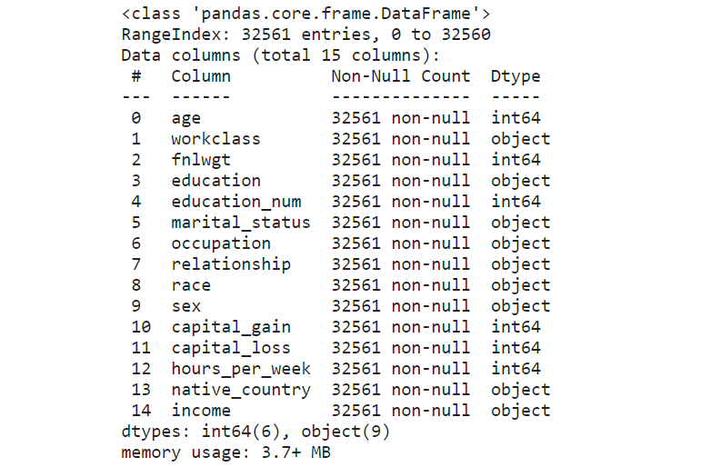

Box plots are useful as they show outliers for integer data types within a data set. An outlier is an observation that is numerically distant from the rest of the data. When reviewing a box plot, an outlier is defined as a data point that is located outside the whiskers of the box plot.

箱形圖很有用，因為它們顯示了數據集中整數數據類型的離群值。 離群值是在數值上與其余數據相距遙遠的觀測值 。 查看箱形圖時，離群值定義為位于箱形圖晶須之外的數據點。

# Use a boxplot to detect any outliers
income_data.boxplot(figsize=(30,6), fontsize=20);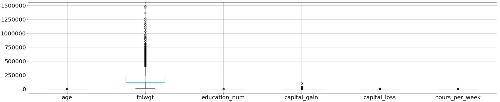

As extracted from the attributes listing in the Census Income Data Set, the feature “fnlwgt” refers to the final weight. It states the number of people the census believes the entry represents. Therefore, this outlier would not be relevant to our analysis and we would proceed to drop this column.

從“ 人口普查收入數據集 ”中的屬性列表中提取的功能“ fnlwgt”是指最終權重。 它指出了人口普查相信該條目所代表的人數。 因此，此異常值與我們的分析無關，我們將繼續刪除此列。

clean_df = income_data.drop(['fnlwgt'], axis=1)
clean_df.info()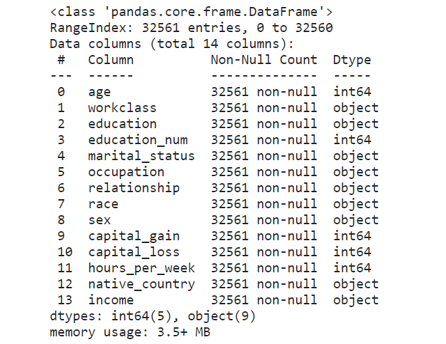

# Select duplicate rows except first occurrence based on all columns
dup_rows = clean_df[clean_df.duplicated()]
dup_rows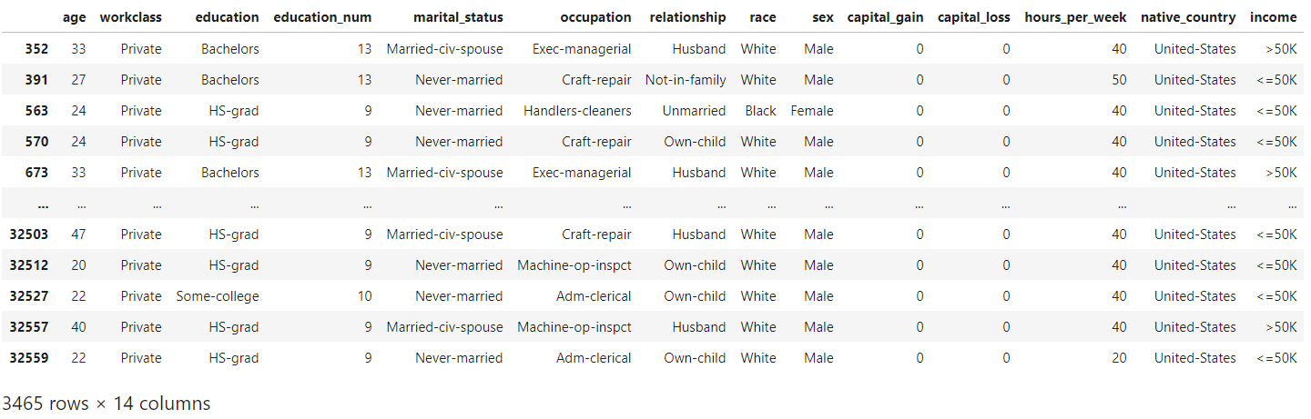

An example of duplicates can be seen in the above rows with the entries “Private” under the “workclass” column. These duplicate rows correspond to samples for different surveyed individuals instead of genuine duplicate rows. As such, we would not remove any duplicated rows to preserve the data for further analysis.

可以在上面的行中看到重復的示例，在“工作類別”列下有條目“私人”。 這些重復的行對應于不同調查對象的樣本，而不是真正的重復行。 因此，我們不會刪除任何重復的行來保留數據以供進一步分析。

標簽編碼 (Label Encoding)

Categorical features are encoded into numerical values using label encoding, to convert each class under the specified feature to a numerical value.

使用標簽編碼將分類要素編碼為數值，以將指定要素下的每個類別轉換為數值。

# Categorical boolean mask
categorical_feature_mask = clean_df.dtypes==object# Filter categorical columns using mask and turn it into a list
categorical_cols = clean_df.columns[categorical_feature_mask].tolist()# Instantiate labelencoder object
le = LabelEncoder()# Apply label encoder on categorical feature columns
clean_df[categorical_cols] = clean_df[categorical_cols].apply(lambda col: le.fit_transform(col))
clean_df[categorical_cols].head(5)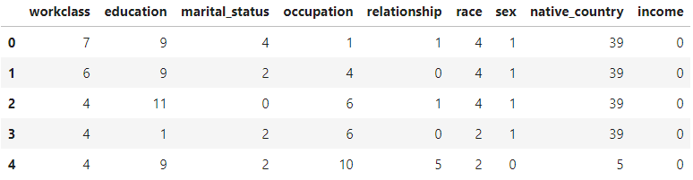

X = clean_df.iloc[:,0:13]  # independent columns - features
y = clean_df.iloc[:,-1]    # target column - income# Distribution of target variable
print(clean_df["income"].value_counts())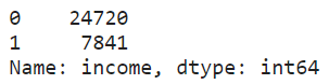

print(clean_df["income"].value_counts(normalize=True))
# 0 for label: <= U$50K
# 1 for label: > U$50K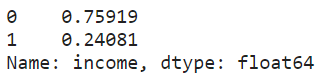

An imbalanced dataset was observed from the above-normalized distribution.

從上述歸一化分布中觀察到不平衡的數據集。

實驗設計 (Design of Experiment)

It would be interesting to see how different factors can affect the performance of each classifier. Let’s consider the following 3 factors:

看看不同的因素如何影響每個分類器的性能會很有趣。 讓我們考慮以下三個因素：

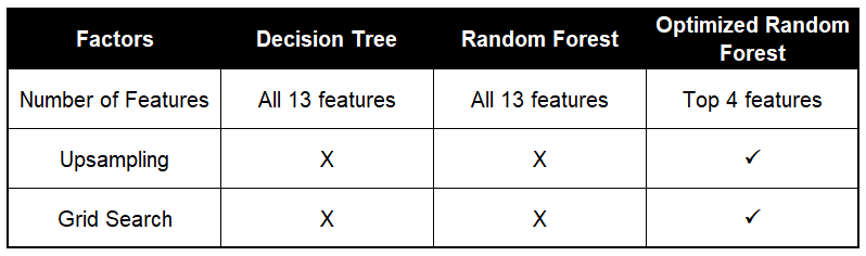
• Number of features: When deciding on the number of features to use for a particular dataset, The Elements of Statistical Learning (section 15.3) states that:

  特征數量：在確定用于特定數據集的特征數量時， 《統計學習的要素》 (第15.3節)指出：

Typically, for a classification problem with p features, √p features are used in each split.

通常，對于具有p個特征的分類問題，在每個拆分中使用√p個特征。

Thus, we would perform feature selection to choose the top 4 features for the modeling of the optimized random forest. With the ideal number of features, it would help to prevent overfitting and improve model interpretability.

因此，我們將執行特征選擇，以選擇用于優化隨機森林建模的前4個特征。 具有理想數量的功能，將有助于防止過度擬合并提高模型的可解釋性。

• Upsampling: An imbalanced dataset would lead to a biased model after training. For this particular dataset, we see a distribution of 76% representing the majority class (ie. income <=U$50K) and the remaining 24% representing the minority class (ie. income >U$50K).

  上采樣：訓練后，不平衡的數據集會導致模型產生偏差。 對于這個特定的數據集，我們看到76％的分布代表多數階層(即，收入<= U $ 50K)，其余24％的分布代表少數群體(即，收入> U $ 50K)。

Upon training of the models, we will have the decision tree and random forest achieving a high classification accuracy belonging to the majority class. To overcome this, we would perform an upsampling of the minority class (ie. income >U$50K) to create a balanced dataset for the optimized random forest model.

訓練模型后，我們將擁有屬于多數類別的，具有較高分類精度的決策樹和隨機森林。 為了克服這個問題，我們將對少數群體(即收入> 5萬美元)進行上采樣，以為優化的隨機森林模型創建一個平衡的數據集。

• Grid search: In order to maximize the performance of the random forest, we can perform a grid search for the best hyperparameters and optimize the random forest model.

  網格搜索：為了最大化隨機森林的性能，我們可以對最佳超參數執行網格搜索并優化隨機森林模型。

資料建模 (Data Modelling)

An initial loading and splitting of the dataset were performed to train and test the decision tree and random forest models, before optimizing the random forest.

在優化隨機森林之前，先對數據集進行初始加載和拆分，以訓練和測試決策樹和隨機森林模型。

X_train_bopt, X_test_bopt, y_train_bopt, y_test_bopt = train_test_split(X, y,test_size = 0.3,random_state = 1)

Standardization of datasets is a common requirement for many machine learning estimators implemented in scikit-learn. The dataset might behave badly if the individual features do not more or less look like standard normally distributed data, ie. Gaussian with zero mean and unit variance.

標準化 對于scikit-learn中實現的許多機器學習估計器，數據集的數量是一個普遍的要求。 如果各個要素看起來或多或少不像標準正態分布數據(即)，則數據集的行為可能會很差。 具有零均值和單位方差的高斯。

# Perform pre-processing to scale numeric features
scale = preprocessing.StandardScaler()
X_train_bopt = scale.fit_transform(X_train_bopt)# Test features are scaled using the scaler computed for the training features
X_test_bopt = scale.transform(X_test_bopt)

模型1：決策樹 (Model 1: Decision Tree)

# Create decision tree classifier
tree = DecisionTreeClassifier(random_state=1)# Fit training data and training labels to decision tree
tree.fit(X_train_bopt, y_train_bopt)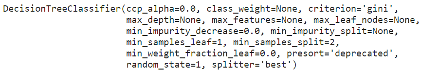

print(f'Decision Tree has {tree.tree_.node_count} nodes with a maximum depth of {tree.tree_.max_depth}.')print(f'Model Accuracy for train data: {tree.score(X_train_bopt, y_train_bopt)}')
print(f'Model Accuracy for test data: {tree.score(X_test_bopt, y_test_bopt)}')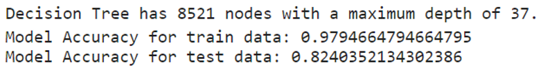

As there was no limit on the depth, the decision tree model was able to classify every training point perfectly to a large extent.

由于深度沒有限制，因此決策樹模型能夠在很大程度上對每個訓練點進行完美分類。

決策樹的可視化 (Visualization of the Decision Tree)

By visualizing the decision tree, it will show each node in the tree which we can use to make new predictions. As the tree is relatively large, the decision tree is plotted below, with a maximum depth of 3.

通過可視化決策樹，它將顯示樹中的每個節點，我們可以使用它們進行新的預測。 由于樹比較大，下面繪制了決策樹，最大深度為3。

# Create and fit decision tree with maximum depth 3
tree = DecisionTreeClassifier(max_depth=3, random_state=1)
tree.fit(X_train_bopt, y_train_bopt)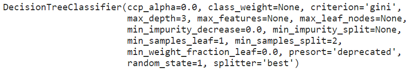

# Plot the decision tree
plt.figure(figsize=(25,10))
decision_tree_plot = plot_tree(tree, feature_names=X.columns, class_names=['<=50K','>50K'], filled=True, rounded=True, fontsize=14)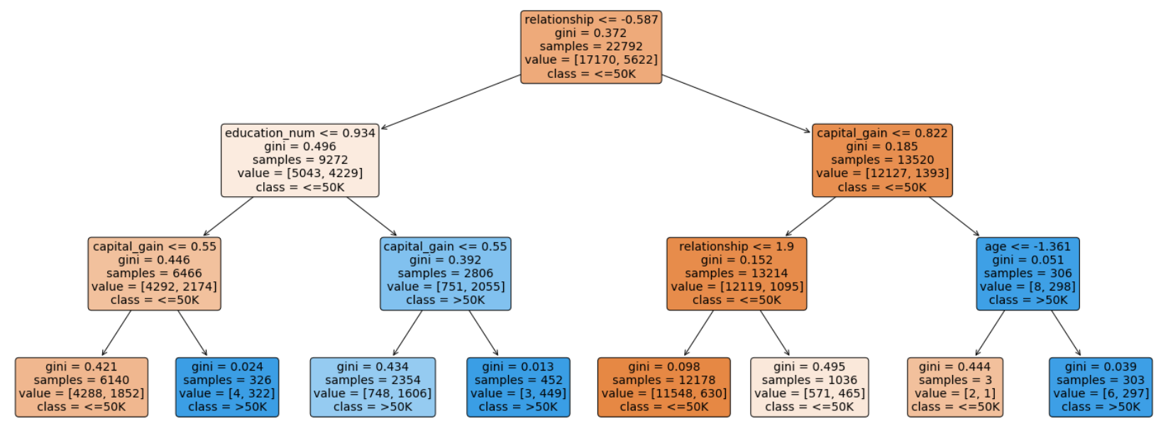

對于每個節點(葉節點除外)，五行表示： (For each of the nodes (except the leaf nodes), the five rows represent:)

1. question asked about the data based on a feature: This determines the way we traverse down the tree for a new data point.

   question asked about the data based on a feature ：這確定了我們遍歷樹以獲取新數據點的方式。

2. gini: The gini impurity of the node represents the probability that a randomly selected sample from a node will be incorrectly classified according to the distribution of samples in the node. The average (weighted by samples) gini impurity decreases with each level of the tree.

   gini ：節點的gini雜質表示從節點中隨機選擇的樣本將根據節點中樣本的分布進行錯誤分類的概率。 樹木的每個水平均會降低吉尼雜質的平均值(按樣品加權)。

3. samples: The number of training observations in the node.

   samples ：節點中訓練觀測的數量。

4. value: The number of samples in the respective classes.

   value ：各個類別中的樣本數。

5. class: The class predicted for all the points in the node if the tree ended at this depth.

   class ：如果樹在此深度處結束，則為節點中所有點預測的類。

The leaf nodes are where the tree makes a prediction. The different colors correspond to the respective classes, with shades ranging from light to dark depending on the gini impurity.

葉子節點是樹進行預測的地方。 不同的顏色對應于各個類別，取決于基尼雜質，陰影的范圍從淺到深。

修剪決策樹 (Pruning the Decision Tree)

Limiting the maximum depth of the decision tree can enable the tree to generalize better to testing data. Although this will lead to reduced accuracy on the training data, it can improve performance on the testing data and provide an objective performance evaluation.

限制決策樹的最大深度可以使決策樹更好地推廣到測試數據。 盡管這將導致訓練數據的準確性降低，但可以提高測試數據的性能并提供客觀的性能評估。

# Create for loop to prune tree
scores = []for i in range(1, 31):tree = DecisionTreeClassifier(random_state=1, max_depth=i)tree.fit(X_train_bopt, y_train_bopt)score = tree.score(X_test_bopt, y_test_bopt)scores.append(tree.score(X_test_bopt, y_test_bopt))# Plot graph to see how individual accuracy scores changes with tree depth
sns.set_context('talk')
sns.set_palette('dark')
sns.set_style('ticks')plt.plot(range(1, 31), scores)
plt.xlabel("Depth of Tree")
plt.ylabel("Scores")
plt.title("Decision Tree Classifier Accuracy")
plt.show()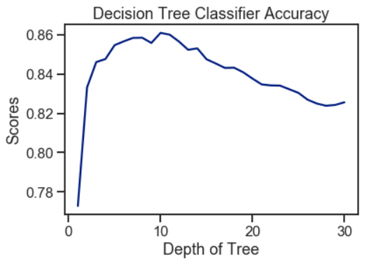

Using the decision tree, a peak of 86% accuracy was achieved with an optimal tree depth of 10. As the depth of the tree increases, the accuracy score decreases gradually. Hence, a deeper tree depth does not reflect a higher accuracy for prediction.

使用決策樹時，最佳樹深度為10時，達到了86％的精度峰值。隨著樹的深度增加，精度得分逐漸降低。 因此，更深的樹深度不能反映更高的預測精度。

模型2：隨機森??林 (Model 2: Random Forest)

包外錯誤評估 (Out-of-Bag Error Evaluation)

The Random Forest Classifier is trained using bootstrap aggregation, where each new tree is fitted from a bootstrap sample of the training observations. The out-of-bag error is the average error for each training observation calculated using predictions from the trees that do not contain the training observation in their respective bootstrap sample. This allows the Random Forest Classifier to be fitted and validated whilst being trained.

使用引導聚合對隨機森林分類器進行訓練，其中從訓練觀測值的引導樣本中擬合出每棵新樹。 袋外誤差是每個訓練觀測值的平均誤差，這些誤差是使用來自在其各自的引導樣本中不包含訓練觀測值的樹的預測所計算出的。 這允許在訓練過程中對隨機森林分類器進行擬合和驗證。

The random forest model was fitted with a range of tree numbers and evaluated on the out-of-bag error for each of the tree’s numbers used.

隨機森林模型配有一系列樹木編號，并針對所使用的每個樹木編號評估了袋外誤差。

# Initialise the random forest estimator
# Set 'warm_start=true' so that more trees are added to the existing model each iteration
RF = RandomForestClassifier(oob_score=True, random_state=1, warm_start=True, n_jobs=-1)oob_list = list()# Iterate through all of the possibilities for the number of trees
for n_trees in [15, 20, 30, 40, 50, 100, 150, 200, 300, 400]:RF.set_params(n_estimators=n_trees)  # Set number of treesRF.fit(X_train_bopt, y_train_bopt)oob_error = 1 - RF.oob_score_ # Obtain the oob erroroob_list.append(pd.Series({'n_trees': n_trees, 'oob': oob_error}))rf_oob_df = pd.concat(oob_list, axis=1).T.set_index('n_trees')ax = rf_oob_df.plot(legend=False, marker='o')
ax.set(ylabel='out-of-bag error',title='Evaluation of Out-of-Bag Error');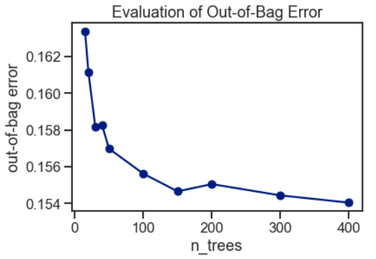

The out-of-bag error appeared to have stabilized around 150 trees.

袋外誤差似乎已穩定在150棵樹附近。

# Create the model with 150 trees
forest = RandomForestClassifier(n_estimators=150, random_state=1, n_jobs=-1)# Fit training data and training labels to forest
forest.fit(X_train_bopt, y_train_bopt)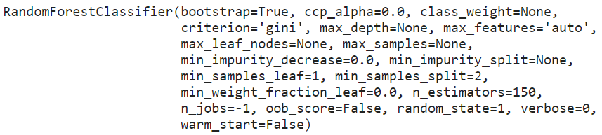

n_nodes = []
max_depths = []for ind_tree in forest.estimators_:n_nodes.append(ind_tree.tree_.node_count)max_depths.append(ind_tree.tree_.max_depth)print(f'Random Forest has an average number of nodes {int(np.mean(n_nodes))} with an average maximum depth of {int(np.mean(max_depths))}.')print(f'Model Accuracy for train data: {forest.score(X_train_bopt, y_train_bopt)}')
print(f'Model Accuracy for test data: {forest.score(X_test_bopt, y_test_bopt)}')

From the above, each decision tree in the random forest has many nodes and is extremely deep. Although each individual decision tree may overfit to a particular subset of the training data, the use of random forest had produced a slightly higher accuracy score for the test data.

綜上所述，隨機森林中的每個決策樹都有許多節點，并且深度非常大。 盡管每個決策樹都可能過度適合訓練數據的特定子集，但是使用隨機森林對測試數據的準確性得分略高。

功能重要性 (Feature Importance)

The feature importance of each feature of the dataset can be obtained by using the feature importance property of the model. Feature importance gives a score for each feature of the data. The higher the score, the more important or relevant the feature is towards the target variable.

可以通過使用模型的特征重要性屬性來獲得數據集的每個特征的特征重要性。 特征重要性為數據的每個特征給出分數。 分數越高，特征對目標變量的重要性或相關性就越高。

Feature importance is an in-built class that comes with Tree-Based Classifiers. We have used the decision tree and random forest to rank the feature importance for the dataset.

功能重要性是基于樹的分類器附帶的內置類。 我們已經使用決策樹和隨機森林對數據集的特征重要性進行排序。

feature_imp = pd.Series(tree.feature_importances_, index=X.columns).sort_values(ascending=False)ax = feature_imp.plot(kind='bar')
ax.set(title='Feature Importance - Decision Trees',ylabel='Relative Importance');feature_imp = pd.Series(forest.feature_importances_, index=X.columns).sort_values(ascending=False)ax = feature_imp.plot(kind='bar')
ax.set(title='Feature Importance - Random Forest',ylabel='Relative Importance');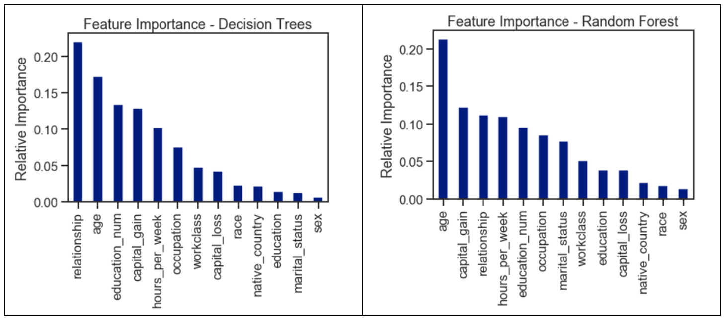

The features were ranked based on their importance considered by the respective classifiers. The values were computed by summing the reduction in Gini Impurity over all of the nodes of the tree in which the feature is used.

根據各個分類器考慮的重要性對功能進行排名。 通過對使用該特征的樹的所有節點上的基尼雜質減少量求和來計算這些值。

使用2種方法進行特征選擇： (Feature Selection using 2 Methods:)

1.單變量選擇 (1. Univariate Selection)

Statistical tests can be used to select those features that have the strongest relationship with the target variable. The scikit-learn library provides the SelectKBest class to be used with a suite of different statistical tests to select a specific number of features. We used the chi-squared (chi2) statistical test for non-negative features to select 10 of the best features from the dataset.

可以使用統計檢驗來選擇與目標變量關系最密切的那些特征 。 scikit-learn庫提供SelectKBest類，該類將與一組不同的統計測試一起使用，以選擇特定數量的功能。 我們使用非負特征的卡方(chi2)統計檢驗從數據集中選擇10個最佳特征。

# Apply SelectKBest class to extract top 10 best features
bestfeatures = SelectKBest(score_func=chi2, k=10)
fit = bestfeatures.fit(X,y)
dfscores = pd.DataFrame(fit.scores_)
dfcolumns = pd.DataFrame(X.columns)# Concatenate two dataframes for better visualization 
featureScores = pd.concat([dfcolumns,dfscores],axis=1)
featureScores.columns = ['Features','Score']  # naming the dataframe columns
print(featureScores.nlargest(10,'Score'))  # print 10 best features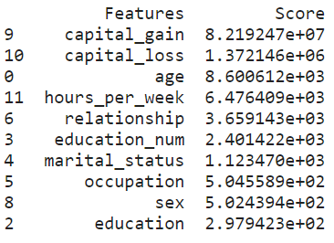

2.具有熱圖的相關矩陣 (2. Correlation Matrix with Heat Map)

Correlation states how the features are related to each other or the target variable. Correlation can be positive (increase in one value of feature increases the value of the target variable) or negative (increase in one value of feature decreases the value of the target variable). A heat map makes it easy to identify which features are most related to the target variable.

關聯說明要素之間如何相互關聯或與目標變量關聯。 相關可以是正的(增加一個特征值增加目標變量的值)或負的(增加一個特征值減少目標變量的值)。 通過熱圖 ，可以輕松識別出哪些特征與目標變量最相關 。

# Obtain correlations of each features in dataset
sns.set(font_scale=1.4)
corrmat = clean_df.corr()
top_corr_features = corrmat.index
plt.figure(figsize=(30,30))# Plot heat map
correlation = sns.heatmap(clean_df[top_corr_features].corr(),annot=True,fmt=".3f",cmap='Blues')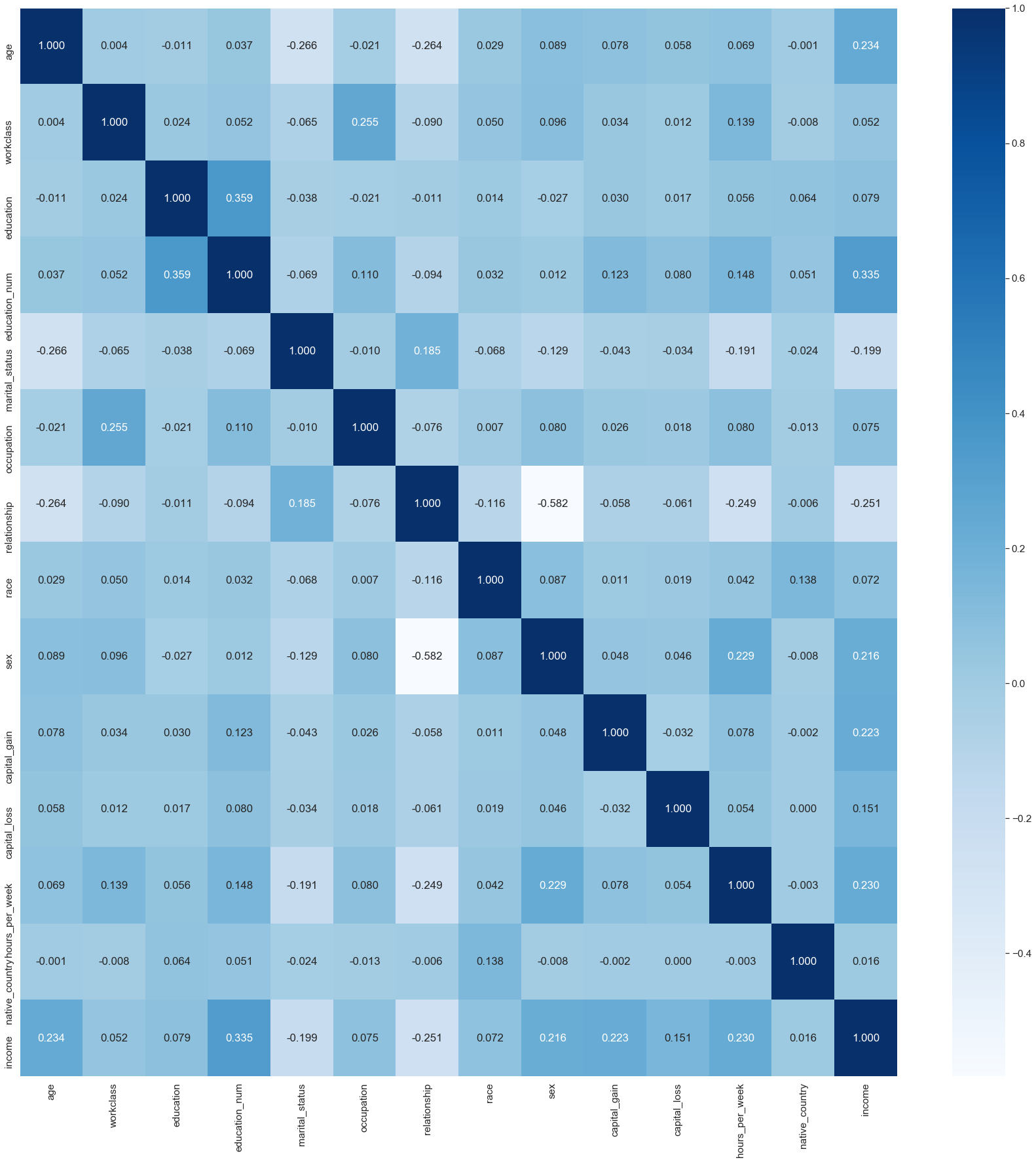

上采樣 (Upsampling)

Upsampling is the process of randomly duplicating observations from the minority class in order to reinforce its signal. There are several heuristics for doing so, but the most common way is to simply resample with replacement.

上采樣是隨機復制少數群體的觀察結果以增強其信號的過程 。 這樣做有幾種啟發式方法，但是最常見的方法是簡單地用替換進行重新采樣。

# Separate majority and minority classes
df_majority = clean_df[clean_df.income==0]
df_minority = clean_df[clean_df.income==1]# Upsample minority class
df_minority_upsampled = resample(df_minority, replace=True,     # sample with replacementn_samples=24720,  # to match majority classrandom_state=1)   # reproducible results# Combine majority class with upsampled minority class
df_upsampled = pd.concat([df_majority, df_minority_upsampled])# Display new class counts
df_upsampled.income.value_counts()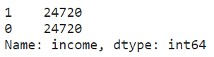

df_upsampled.income.value_counts(normalize=True)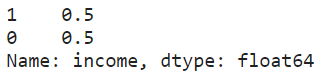

Now that the dataset has been balanced, we are ready to split and scale this dataset for training and testing using the optimized random forest model.

現在數據集已經達到平衡，我們已經準備好使用優化的隨機森林模型拆分和縮放該數據集，以進行訓練和測試。

X_upsamp = df_upsampled[feature_cols]
y_upsamp = df_upsampled['income']X_train, X_test, y_train, y_test = train_test_split(X_upsamp, y_upsamp, test_size = 0.3, random_state = 1)# Perform pre-processing to scale numeric features
scale = preprocessing.StandardScaler()
X_train = scale.fit_transform(X_train)# Test features are scaled using the scaler computed for the training features
X_test = scale.transform(X_test)

通過網格搜索進行隨機森林優化 (Random Forest Optimization through Grid Search)

Grid search is an exhaustive search over specified parameter values for an estimator. It selects combinations of hyperparameters from a grid, evaluates them using cross-validation on the training data, and returns the values that perform the best.

網格搜索是對估計器的指定參數值的詳盡搜索 。 它從網格中選擇超參數組合，對訓練數據使用交叉驗證對它們進行評估，然后返回性能最佳的值。

We have selected the following model parameters for the grid search:

我們為網格搜索選擇了以下模型參數 ：

• n_estimators: The number of trees in the forest.

  n_estimators：森林中樹木的數量。

• max_depth: The maximum depth of the tree.

  max_depth：樹的最大深度。

• min_samples_split: The minimum number of samples required to split an internal node.

  min_samples_split：拆分內部節點所需的最小樣本數。

# Set the model parameters for grid search
model_params = {'n_estimators': [150, 200, 250, 300],'max_depth': [15, 20, 25],'min_samples_split': [2, 4, 6]}# Create random forest classifier model
rf_model = RandomForestClassifier(random_state=1)# Set up grid search meta-estimator
gs = GridSearchCV(rf_model, model_params,n_jobs=-1, scoring='roc_auc', cv=3)# Train the grid search meta-estimator to find the best model
best_model = gs.fit(X_train, y_train)# Print best set of hyperparameters
from pprint import pprint
pprint(best_model.best_estimator_.get_params())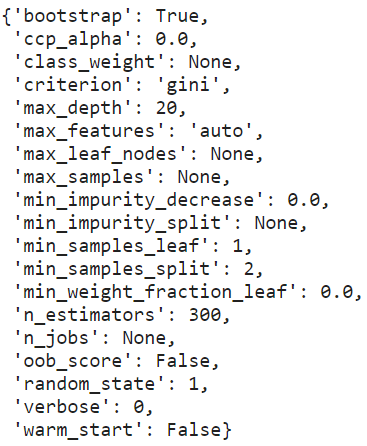

Based on the grid search, the best hyperparameter values were not the defaults. This shows the importance of tuning a model for a specific dataset. Each dataset will have different characteristics, and the model that does best on one dataset will not necessarily do the best across all datasets.

基于網格搜索，最佳超參數值不是默認值。 這表明為特定數據集調整模型的重要性。 每個數據集將具有不同的特征，并且在一個數據集上表現最佳的模型不一定會在所有數據集上表現最佳。

使用最佳模型優化隨機森林 (Use the Best Model to Optimize Random Forest)

n_nodes = []
max_depths = []for ind_tree in best_model.best_estimator_:n_nodes.append(ind_tree.tree_.node_count)max_depths.append(ind_tree.tree_.max_depth)print(f'The optimized random forest has an average number of nodes {int(np.mean(n_nodes))} with an average maximum depth of {int(np.mean(max_depths))

The best maximum depth was not unlimited, this indicates that restricting the maximum depth of the individual decision trees can improve the cross validation performance of the random forest.

最佳最大深度不是無限的，這表明限制單個決策樹的最大深度可以提高隨機森林的交叉驗證性能。

print(f'Model Accuracy for train data: {best_model.score(X_train, y_train)}')
print(f'Model Accuracy for test data: {best_model.score(X_test, y_test)}')

Although the performance achieved by the optimized model was slightly below that of the decision tree and default model, the gap between the model accuracy obtained for both the train data and test data was minimized (~4%). This represents a good fit of the learning curve where a high accuracy rate was achieved by using the trained model on the test data.

盡管通過優化模型獲得的性能略低于決策樹和默認模型，但是針對火車數據和測試數據獲得的模型精度之間的差距已最小化(?4％)。 這代表了學習曲線的良好擬合，其中通過在測試數據上使用經過訓練的模型可以實現較高的準確率。

模型的性能評估 (Performance Evaluation of Models)

# Predict target variables (ie. labels) for each classifer
dt_classifier_name = ["Decision Tree"]
dt_predicted_labels = tree.predict(X_test_bopt)rf_classifier_name = ["Random Forest"]
rf_predicted_labels = forest.predict(X_test_bopt)best_model_classifier_name = ["Optimized Random Forest"]
best_model_predicted_labels = best_model.predict(X_test)

1.分類報告 (1. Classification Report)

The classification report shows a representation of the main classification metrics on a per-class basis and gives a deeper intuition of the classifier behavior over global accuracy, which can mask functional weaknesses in one class of a multi-class problem. The metrics are defined in terms of true and false positives, and true and false negatives.

分類報告顯示了每個分類的主要分類指標，并給出了分類器行為相對于全局準確性的更直觀認識，這可以掩蓋一類多分類問題中的功能弱點。 度量是根據正確和錯誤肯定以及正確和錯誤否定來定義的。

Precision is the ability of a classifier not to label an instance positive that is actually negative. For each class, it is defined as the ratio of true positives to the sum of true and false positives.

精度是分類器不標記實際為負的實例正的能力。 對于每個類別，它定義為真陽性與真假陽性之和的比率。

For all instances classified positive, what percent was correct?

對于所有歸類為陽性的實例，正確的百分比是多少？

Recall is the ability of a classifier to find all positive instances. For each class, it is defined as the ratio of true positives to the sum of true positives and false negatives.

回憶是分類器查找所有正實例的能力。 對于每個類別，它定義為真陽性與真陽性與假陰性總和之比。

For all instances that were actually positive, what percent was classified correctly?

對于所有實際為正的實例，正確分類的百分比是多少？

The F1-score is a weighted harmonic mean of precision and recall such that the best score is 1.0 and the worst is 0.0. Generally, F1-scores are lower than accuracy measures as they embed precision and recall into their computation. As a rule of thumb, the weighted average of the F1-score should be used to compare classifier models, not global accuracy.

F1分數是精確度和召回率的加權諧波平均值，因此最佳分數是1.0，最差分數是0.0。 通常，F1分數將精度和召回率嵌入到計算中，因此它們比精度度量要低。 根據經驗，應該使用F1分數的加權平均值來比較分類器模型，而不是整體精度。

Support is the number of actual occurrences of the class in the specified dataset. Imbalanced support in the training data may indicate structural weaknesses in the reported scores of the classifier and could indicate the need for stratified sampling or re-balancing. Support does not change between models but instead diagnoses the evaluation process.

支持是指定數據集中該類的實際出現次數。 訓練數據中支持不平衡可能表明分類器報告的分數存在結構性缺陷，并且可能表明需要分層抽樣或重新平衡。 支持在模型之間不會改變，而是診斷評估過程。

print("Classification Report for",dt_classifier_name, " :\n ",metrics.classification_report(y_test_bopt, dt_predicted_labels, target_names=['Income <= U$50K','Income > U$50K']))print("Classification Report for ",rf_classifier_name, " :\n ",metrics.classification_report(y_test_bopt, rf_predicted_labels,target_names=['Income <= U$50K','Income > U$50K']))print("Classification Report for ",best_model_classifier_name, " :\n ",metrics.classification_report(y_test,best_model_predicted_labels,target_names=['Income <= U$50K','Income > U$50K']))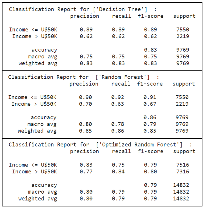

The optimized random forest has performed well in the above metrics. In particular, with upsampling performed to maintain a balanced dataset, a significant observation was noted in the minority class (ie. label ‘1’ representing income > U$50K), where recall scores had improved 35%, from 0.62 to 0.84, by using the optimized random forest model.

經過優化的隨機森林在上述指標中表現良好。 尤其是，為了保持數據集的平衡而進行了上采樣， 在少數族裔類別中觀察到了顯著的結果(即標簽“ 1”代表收入> 5萬美元)， 召回得分提高了35％，從0.62提高到0.84，使用優化的隨機森林模型。

With a higher precision and recall scores, the optimized random forest model was able to correctly label instances that were indeed positive. Out of these instances which were actually positive, the optimized random forest model had classified them correctly to a large extent. This directly translates into a higher F1-score as a weighted harmonic mean of precision and recall.

優化的隨機森林模型具有更高的精度和召回得分 ，能夠正確標記確實為陽性的實例。 在這些實際為陽性的實例中，優化后的隨機森林模型在很大程度上將它們正確分類。 這直接轉化為更高的F1得分，作為精確度和召回率的加權諧波平均值。

2.混淆矩陣 (2. Confusion Matrix)

The confusion matrix takes a fitted scikit-learn classifier and a set of test x and y values and returns a report showing how each of the test values predicted classes compare to their actual classes. These provide similar information as what is available in a classification report, but rather than top-level scores, they provide deeper insight into the classification of individual data points.

混淆矩陣采用適合的scikit-learn分類器和一組測試x和y值，并返回報告，顯示每個預測值預測類與實際類的比較。 這些提供的信息與分類報告中提供的信息類似，但是它們不是頂級分數，而是提供了對單個數據點分類的更深入了解。

print("Confusion Matrix for",dt_classifier_name)
skplt.metrics.plot_confusion_matrix(y_test_bopt, dt_predicted_labels, normalize=True)
plt.show()print("Confusion Matrix for",rf_classifier_name)
skplt.metrics.plot_confusion_matrix(y_test_bopt, rf_predicted_labels, normalize=True)
plt.show()print("Confusion Matrix for",best_model_classifier_name)
skplt.metrics.plot_confusion_matrix(y_test, best_model_predicted_labels, normalize=True)
plt.show()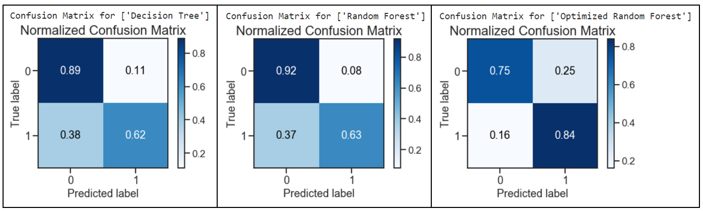

The optimized random forest had performed well with a decrease in the Type 2 Error: False Negatives (predicted income <= U$50K but actually income > U$50K). A remarkable decrease of 58% was obtained from a score of 0.38 to 0.16 when comparing the results for decision tree against the optimized random forest.

經過優化的隨機森林表現良好，并且減少了Type 2錯誤：False Negatives (預期收入<= 5萬美元，但實際收入> 5萬美元)。 將決策樹的結果與優化的隨機森林進行比較時， 得分從0.38下降到0.16 ， 下降了58％ 。

However, the Type 1 Error: False Positives (predicted > U$50K but actually <= U$50K) had approximately tripled, from 0.08 to 0.25, by comparing the optimized random forest with the default random forest model.

但是，通過將優化后的隨機森林與默認隨機森林模型進行比較， 類型1錯誤：誤報 (預測為> 5萬美元，但實際<= 5萬美元) 大約增加了三倍，從0.08到0.25 。

Overall, the impact of having more false positives was mitigated with a notable decrease in false negatives. With a good outcome of the test values predicted classes as compared to their actual classes, the confusion matrix results for the optimized random forest had outperformed the other models.

總體而言，誤報率明顯下降，減輕了更多誤報率的影響。 測試值預測類比其實際類具有更好的結果，優化隨機森林的混淆矩陣結果優于其他模型。

3.精確調用曲線 (3. Precision-Recall Curve)

Precision-Recall curve is a metric used to evaluate a classifier’s quality. The precision-recall curve shows the trade-off between precision, a measure of result relevancy, and recall, a measure of how many relevant results are returned. A large area under the curve represents both high recall and precision, the best-case scenario for a classifier, showing a model that returns accurate results for the majority of classes it selects.

精確召回曲線是用于評估分類器質量的指標。 精度調用曲線顯示了精度(即結果相關性的度量)和召回率(即返回了多少相關結果的度量)之間的權衡。 曲線下的較大區域代表了較高的查全率和精度，這是分類器的最佳情況，它顯示了一個模型，該模型針對選擇的大多數類別返回準確的結果。

fig, axList = plt.subplots(ncols=3)
fig.set_size_inches(21,6)# Plot the Precision-Recall curve for Decision Tree   
ax = axList[0]
dt_predicted_proba = tree.predict_proba(X_test_bopt)
precision, recall, _ = precision_recall_curve(y_test_bopt, dt_predicted_proba[:,1])
ax.plot(recall, precision,color='black')
ax.set(xlabel='Recall', ylabel='Precision', xlim=[0, 1], ylim=[0, 1],title='Precision-Recall Curve - Decision Tree')
ax.grid(True)# Plot the Precision-Recall curve for Random Forest
ax = axList[1]
rf_predicted_proba = forest.predict_proba(X_test_bopt)
precision, recall, _ = precision_recall_curve(y_test_bopt, rf_predicted_proba[:,1])
ax.plot(recall, precision,color='green')
ax.set(xlabel='Recall', ylabel='Precision', xlim=[0, 1], ylim=[0, 1],title='Precision-Recall Curve - Random Forest')
ax.grid(True)# Plot the Precision-Recall curve for Optimized Random Forest
ax = axList[2]
best_model_predicted_proba = best_model.predict_proba(X_test)
precision, recall, _ = precision_recall_curve(y_test, best_model_predicted_proba[:,1])
ax.plot(recall, precision,color='blue')
ax.set(xlabel='Recall', ylabel='Precision', xlim=[0, 1], ylim=[0, 1],title='Precision-Recall Curve - Optimised Random Forest')
ax.grid(True)
plt.tight_layout()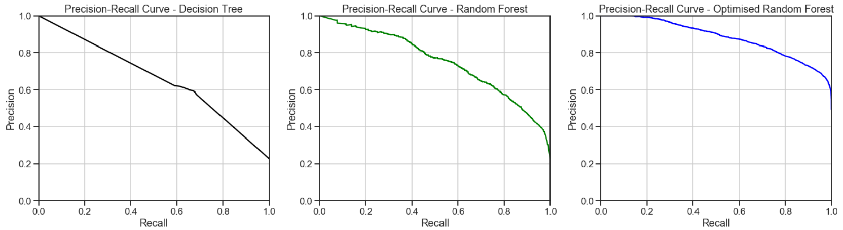

The optimized random forest classifier achieved a higher area under the precision-recall curve. This represents high recall and precision scores, where high precision relates to a low false-positive rate, and a high recall relates to a low false-negative rate. High scores in both showed that the optimized random forest classifier had returned accurate results (high precision), as well as a majority of all positive results (high recall).

優化的隨機森林分類器在精確召回曲線下獲得了更大的面積。 這代表了較高的查全率和精確度分數，其中高精度與低假陽性率相關，而高查全率與較低的假陰性率相關。 兩者均獲得高分，表明優化后的隨機森林分類器已返回準確結果(高精度)，以及大部分積極結果(高召回率)。

4. ROC曲線和AUC (4. ROC Curve and AUC)

A Receiver Operating Characteristic (“ROC”)/Area Under the Curve (“AUC”) plot allows the user to visualize the trade-off between the classifier’s sensitivity and specificity.

接收器工作特征(“ ROC”)/曲線下面積(“ AUC”)曲線圖使用戶可以直觀地看到分類器的靈敏度和特異性之間的權衡。

The ROC is a measure of a classifier’s predictive quality that compares and visualizes the trade-off between the model’s sensitivity and specificity. When plotted, a ROC curve displays the true positive rate on the Y axis and the false positive rate on the X axis on both a global average and per-class basis. The ideal point is therefore the top-left corner of the plot: false positives are zero and true positives are one.

ROC是對分類器預測質量的一種度量，它比較并可視化模型的敏感性和特異性之間的權衡。 繪制時，ROC曲線在全局平均值和每個類別的基礎上，在Y軸上顯示真實的陽性率，在X軸上顯示假的陽性率。 因此理想點是圖的左上角：假陽性為零，真陽性為一。

AUC is a computation of the relationship between false positives and true positives. The higher the AUC, the better the model generally is. However, it is also important to inspect the “steepness” of the curve, as this describes the maximization of the true positive rate while minimizing the false positive rate.

AUC是假陽性和真陽性之間的關系的計算。 AUC越高，模型通常越好。 但是，檢查曲線的“陡度”也很重要，因為這描述了真實陽性率的最大化，同時最小化了陽性陽性率。

fig, axList = plt.subplots(ncols=3)
fig.set_size_inches(21,6)# Plot the ROC-AUC curve for Decision Tree
ax = axList[0]
dt = tree.fit(X_train_bopt, y_train_bopt.values.ravel()) 
dt_predicted_label_r = dt.predict_proba(X_test_bopt)def plot_auc(y, probs):fpr, tpr, threshold = roc_curve(y, probs[:,1])auc = roc_auc_score(y_test_bopt, dt_predicted_labels)ax.plot(fpr, tpr, color = 'black', label = 'AUC_Decision Tree = %0.2f' % auc)ax.plot([0, 1], [0, 1],'r--')ax.legend(loc = 'lower right')ax.set(xlabel='False Positive Rate',ylabel='True Positive Rate',xlim=[0, 1], ylim=[0, 1],title='ROC curve')       plot_auc(y_test_bopt, dt_predicted_label_r)
ax.grid(True)# Plot the ROC-AUC curve for Random Forest
ax = axList[1]
rf = forest.fit(X_train_bopt, y_train_bopt.values.ravel()) 
rf_predicted_label_r = rf.predict_proba(X_test_bopt)def plot_auc(y, probs):fpr, tpr, threshold = roc_curve(y, probs[:,1])auc = roc_auc_score(y_test_bopt, rf_predicted_labels)ax.plot(fpr, tpr, color = 'green', label = 'AUC_Random Forest = %0.2f' % auc)ax.plot([0, 1], [0, 1],'r--')ax.legend(loc = 'lower right')ax.set(xlabel='False Positive Rate',ylabel='True Positive Rate',xlim=[0, 1], ylim=[0, 1],title='ROC curve') plot_auc(y_test_bopt, rf_predicted_label_r);
ax.grid(True)# Plot the ROC-AUC curve for Optimized Random Forest
ax = axList[2]
best_model = best_model.fit(X_train, y_train.values.ravel()) 
best_model_predicted_label_r = best_model.predict_proba(X_test)def plot_auc(y, probs):fpr, tpr, threshold = roc_curve(y, probs[:,1])auc = roc_auc_score(y_test, best_model_predicted_labels)ax.plot(fpr, tpr, color = 'blue', label = 'AUC_Optimised Random Forest = %0.2f' % auc)ax.plot([0, 1], [0, 1],'r--')ax.legend(loc = 'lower right')ax.set(xlabel='False Positive Rate',ylabel='True Positive Rate',xlim=[0, 1], ylim=[0, 1],title='ROC curve') plot_auc(y_test, best_model_predicted_label_r);
ax.grid(True)
plt.tight_layout()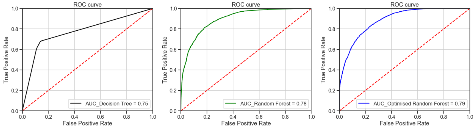

All the models had outperformed the baseline guess with the optimized random forest achieving the best AUC results. Thus, indicating that the optimized random forest is a better classifier.

所有模型均優于基線猜測，優化的隨機森林獲得了最佳的AUC結果。 因此，表明優化的隨機森林是更好的分類器。

5.校準曲線 (5. Calibration Curve)

When performing classification, one often wants to predict not only the class label, but also the associated probability. This probability gives some kind of confidence on the prediction. Thus, the calibration plot is useful for determining whether predicted probabilities can be interpreted directly as an confidence level.

在進行分類時，人們經常不僅要預測分類標簽，還要預測相關的概率。 這種可能性使預測具有某種信心。 因此，校準圖可用于確定預測的概率是否可以直接解釋為置信度。

# Plot calibration curves for a set of classifier probability estimates.
tree = DecisionTreeClassifier()
forest = RandomForestClassifier()tree_probas = tree.fit(X_train_bopt, y_train_bopt).predict_proba(X_test_bopt)
forest_probas = forest.fit(X_train_bopt, y_train_bopt).predict_proba(X_test_bopt)probas_list = [tree_probas, forest_probas]
clf_names = ['Decision Tree','Random Forest']skplt.metrics.plot_calibration_curve(y_test_bopt, probas_list, clf_names,figsize=(10,6))
plt.show()

# Plot calibration curves for a set of classifier probability estimates.
best_model = RandomForestClassifier()best_model_probas = best_model.fit(X_train, y_train).predict_proba(X_test)probas_list = [best_model_probas]
clf_names = ['Optimized Random Forest']skplt.metrics.plot_calibration_curve(y_test, probas_list, clf_names, cmap='winter', figsize=(10,6))
plt.show()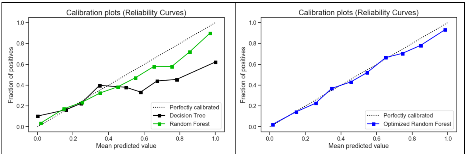

Compared to the other two models, the calibration plot for the optimized random forest was the closest to being perfectly calibrated. Hence, the optimized random forest was more reliable and better able to generalize to new data.

與其他兩個模型相比，優化后的隨機森林的校準圖最接近于完美校準。 因此，優化后的隨機森林更加可靠，能夠更好地推廣到新數據。

結論 (Conclusion)

The optimized random forest had a better generalization performance on the testing set with reduced variance as compared to the other models. Decision trees tend to overfit and pruning helped to reduce variance to a point. The random forest addressed the shortcomings of decision trees with a strong modeling technique which was more robust than a single decision tree.

與其他模型相比， 優化后的隨機森林在測試集上具有更好的泛化性能 ，并且方差減小。 決策樹傾向于過度擬合，而修剪有助于將方差降低到一定程度。 隨機森林使用強大的建模技術解決了決策樹的缺點，該技術比單個決策樹更強大。

The use of optimization for random forest had a significant impact on the results with the following 3 factors being considered:

對隨機森林的優化使用對結果有重大影響，考慮了以下三個因素：

1. Feature selection to chose the ideal number of features to prevent overfitting and improve model interpretability

   選擇特征以選擇理想數量的特征，以防止過度擬合并提高模型的可解釋性

2. Upsampling of the minority class to create a balanced dataset

   少數類的上采樣以創建平衡的數據集

3. Grid search to select the best hyper-parameters to maximize model performance

   網格搜索以選擇最佳超參數以最大化模型性能

Lastly, the results were also attributed by the unique quality of random forest, where it adds additional randomness to the model while growing the trees. Instead of searching for the most important feature while splitting a node, it searches for the best feature among a random subset of features. This results in a wide diversity that generally results in a better model for classification problems.

最后，結果還歸因于隨機森林的獨特質量，即在樹木生長時為模型增加了額外的隨機性。 它不是在分割節點時搜索最重要的特征，而是在特征的隨機子集中搜索最佳特征 。 這導致了廣泛的多樣性，通常可以為分類問題提供更好的模型。