Recommendation systems are becoming increasingly important in today’s hectic world. People are always in the lookout for products/services that are best suited for them. Therefore, the recommendation systems are important as they help them make the right choices, without having to expend their cognitive resources.

在當今繁忙的世界中，推薦系統變得越來越重要。 人們總是在尋找最適合他們的產品/服務。 因此，推薦系統非常重要，因為它們可以幫助他們做出正確的選擇，而不必花費他們的認知資源。

In this blog, we will understand the basics of Recommendation Systems and learn how to build a Movie Recommendation System using collaborative filtering by implementing the K-Nearest Neighbors algorithm. We will also predict the rating of the given movie based on its neighbors and compare it with the actual rating.

在此博客中，我們將了解推薦系統的基礎知識，并學習如何通過實現K最近鄰居算法使用協作過濾來構建電影推薦系統。 我們還將根據給定電影的鄰居來預測給定電影的收視率，并將其與實際收視率進行比較。

推薦系統的類型 (Types of Recommendation Systems)

Recommendation systems can be broadly classified into 3 types —

推薦系統大致可分為3種類型-

1. Collaborative Filtering
   協同過濾
2. Content-Based Filtering
   基于內容的過濾
3. Hybrid Recommendation Systems
   混合推薦系統

協同過濾 (Collaborative Filtering)

This filtering method is usually based on collecting and analyzing information on user’s behaviors, their activities or preferences, and predicting what they will like based on the similarity with other users. A key advantage of the collaborative filtering approach is that it does not rely on machine analyzable content and thus it is capable of accurately recommending complex items such as movies without requiring an “understanding” of the item itself.

這種過濾方法通常基于收集和分析有關用戶的行為，他們的活動或偏好的信息，并基于與其他用戶的相似性來預測他們的需求。 協作過濾方法的主要優勢在于它不依賴于機器可分析的內容，因此能夠準確地推薦諸如電影之類的復雜項目，而無需“了解”項目本身。

Further, there are several types of collaborative filtering algorithms —

此外，協作過濾算法有幾種類型-

• User-User Collaborative Filtering: Try to search for lookalike customers and offer products based on what his/her lookalike has chosen.

  用戶-用戶協作過濾：嘗試搜索相似的客戶并根據他/她的相似選擇提供產品。

• Item-Item Collaborative Filtering: It is very similar to the previous algorithm, but instead of finding a customer lookalike, we try finding item lookalike. Once we have item lookalike matrix, we can easily recommend alike items to a customer who has purchased an item from the store.

  物料-物料協同過濾：它與先前的算法非常相似，但是我們沒有找到相似的客戶，而是嘗試尋找相似的物料。 一旦有了商品相似矩陣，我們就可以輕松地向從商店購買商品的顧客推薦相同商品。

• Other algorithms: There are other approaches like market basket analysis, which works by looking for combinations of items that occur together frequently in transactions.

  其他算法：還有其他方法，例如市場籃分析，其作用是查找交易中經常出現的物品組合。

基于內容的過濾 (Content-based filtering)

These filtering methods are based on the description of an item and a profile of the user’s preferred choices. In a content-based recommendation system, keywords are used to describe the items, besides, a user profile is built to state the type of item this user likes. In other words, the algorithms try to recommend products that are similar to the ones that a user has liked in the past.

這些過濾方法基于項目的描述和用戶偏好選擇的配置文件。 在基于內容的推薦系統中，關鍵字用于描述項目，此外，還建立了一個用戶資料來說明該用戶喜歡的項目的類型。 換句話說，算法嘗試推薦與用戶過去喜歡的產品相似的產品。

混合推薦系統 (Hybrid Recommendation Systems)

Recent research has demonstrated that a hybrid approach, combining collaborative filtering and content-based filtering could be more effective in some cases. Hybrid approaches can be implemented in several ways, by making content-based and collaborative-based predictions separately and then combining them, by adding content-based capabilities to a collaborative-based approach (and vice versa), or by unifying the approaches into one model.

最近的研究表明，將協作過濾和基于內容的過濾相結合的混合方法在某些情況下可能更有效。 可以通過幾種方式來實現混合方法，方法是分別進行基于內容的預測和基于協作的預測，然后將它們組合在一起，將基于內容的功能添加到基于協作的方法中(反之亦然)，或者將這些方法統一為一個方法模型。

Netflix is a good example of the use of hybrid recommender systems. The website makes recommendations by comparing the watching and searching habits of similar users (i.e. collaborative filtering) as well as by offering movies that share characteristics with films that a user has rated highly (content-based filtering).

Netflix是使用混合推薦系統的一個很好的例子。 該網站通過比較相似用戶的觀看和搜索習慣(即協作過濾)，以及通過提供與用戶評價很高的電影具有相同特征的電影(基于內容的過濾)來提供建議。

Now that we’ve got a basic intuition of Recommendation Systems, let’s start with building a simple Movie Recommendation System in Python.

現在，我們已經有了“推薦系統”的基本知識，讓我們從用Python構建一個簡單的電影推薦系統開始。

Find the Python notebook with the entire code along with the dataset and all the illustrations here.

在此處找到帶有完整代碼以及數據集和所有插圖的Python筆記本。

TMDb —電影數據庫 (TMDb — The Movie Database)

The Movie Database (TMDb) is a community built movie and TV database which has extensive data about movies and TV Shows. Here are the stats —

電影數據庫(TMDb)是社區建立的電影和電視數據庫，其中包含有關電影和電視節目的大量數據。 以下是統計資料-

For simplicity and easy computation, I have used a subset of this huge dataset which is the TMDb 5000 dataset. It has information about 5000 movies, split into 2 CSV files.

為了簡化計算，我使用了這個龐大的數據集的一個子集，即TMDb 5000數據集。 它具有約5000部電影的信息，分為2個CSV文件。

• tmdb_5000_movies.csv: Contains information like the score, title, date_of_release, genres, etc.

  tmdb_5000_movies.csv：包含諸如樂譜，標題，發行日期，類型等信息。

• tmdb_5000_credits.csv: Contains information of the cast and crew for each movie.

  tmdb_5000_credits.csv：包含每個電影的演員和劇組信息。

The link to the Dataset is here.

數據集的鏈接在這里 。

第1步-導入數據集 (Step 1 — Import the dataset)

Import the required Python libraries like Pandas, Numpy, Seaborn and Matplotlib. Then import the CSV files using read_csv() function predefined in Pandas.

導入所需的Python庫，例如Pandas，Numpy，Seaborn和Matplotlib。 然后使用Pandas中預定義的read_csv()函數導入CSV文件。

movies = pd.read_csv('../input/tmdb-movie-metadata/tmdb_5000_movies.csv')
credits = pd.read_csv('../input/tmdb-movie-metadata/tmdb_5000_credits.csv')

第2步-數據探索和清理 (Step 2 — Data Exploration and Cleaning)

We will initially use the head(), describe() function to view the values and structure of the dataset, and then move ahead with cleaning the data.

我們將首先使用head() ， describe()函數查看數據集的值和結構，然后繼續清理數據。

movies.head()

movies.describe()

Similarly, we can get an intuition of the credits dataframe and get an output as follows —

同樣，我們可以直觀地了解信用數據框架，并獲得如下輸出：

Checking the dataset, we can see that genres, keywords, production_companies, production_countries, spoken_languages are in the JSON format. Similarly in the other CSV file, cast and crew are in the JSON format. Now let's convert these columns into a format that can be easily read and interpreted. We will convert them into strings and later convert them into lists for easier interpretation.

檢查數據集，我們可以看到流派，關鍵字，production_companies，production_countries，speaked_languages為JSON格式。 同樣，在其他CSV文件中，演員和船員均采用JSON格式。 現在，讓我們將這些列轉換為易于閱讀和解釋的格式。 我們將它們轉換為字符串，然后將它們轉換為列表，以方便解釋。

The JSON format is like a dictionary (key:value) pair embedded in a string. Generally, parsing the data is computationally expensive and time consuming. Luckily this dataset doesn’t have that complicated structure. A basic similarity between the columns is that they have a name key, which contains the values that we need to collect. The easiest way to do so parse through the JSON and check for the name key on each row. Once the name key is found, store the value of it into a list and replace the JSON with the list.

JSON格式就像嵌入在字符串中的字典(鍵：值)對。 通常，解析數據在計算上是昂貴且費時的。 幸運的是，該數據集沒有那么復雜的結構。 列之間的基本相似之處在于它們具有名稱鍵，其中包含我們需要收集的值。 最簡單的方法是通過JSON解析并檢查每一行上的名稱鍵。 找到名稱鍵后，將其值存儲在列表中，然后用列表替換JSON。

But we cannot directly parse this JSON as it has to be decoded first. For this we use the json.loads() method, which decodes it into a list. We can then parse through this list to find the desired values. Let's look at the proper syntax below.

但是我們無法直接解析此JSON，因為必須先對其進行解碼。 為此，我們使用json.loads()方法，將其解碼為列表。 然后，我們可以解析此列表以找到所需的值。 讓我們看看下面的正確語法。

# changing the genres column from json to string
movies['genres'] = movies['genres'].apply(json.loads)
for index,i in zip(movies.index,movies['genres']):
    list1 = []
    for j in range(len(i)):
        list1.append((i[j]['name'])) # the key 'name' contains the name of the genre
    movies.loc[index,'genres'] = str(list1)

In a similar fashion, we will convert the JSON to a list of strings for the columns: keywords, production_companies, cast, and crew. We will check if all the required JSON columns have been converted to strings using movies.iloc[index]

以類似的方式，我們將JSON轉換為以下列的字符串列表：關鍵字，production_companies，cast和crew。 我們將檢查是否所有必需的JSON列都已使用movie.iloc [index]轉換為字符串。

第3步-合并2個CSV文件 (Step 3 — Merge the 2 CSV files)

We will merge the movies and credits dataframes and select the columns which are required and have a unified movies dataframe to work on.

我們將合并電影和片數數據框，然后選擇所需的列并使用統一的電影數據框。

movies = movies.merge(credits, left_on='id', right_on='movie_id', how='left')
movies = movies[['id', 'original_title', 'genres', 'cast', 'vote_average', 'director', 'keywords']]

We can check the size and attributes of movies like this —

我們可以像這樣檢查電影的大小和屬性-

步驟4 —使用“類型”列 (Step 4 — Working with the Genres column)

We will clean the genre column to find the genre_list

我們將清理genre列以找到genre_list

movies['genres'] = movies['genres'].str.strip('[]').str.replace(' ','').str.replace("'",'')
movies['genres'] = movies['genres'].str.split(',')

Let’s plot the genres in terms of their occurrence to get an insight of movie genres in terms of popularity.

讓我們根據流派的出現來繪制流派，以從流行度角度了解電影流派。

plt.subplots(figsize=(12,10))
list1 = []
for i in movies['genres']:
    list1.extend(i)
ax = pd.Series(list1).value_counts()[:10].sort_values(ascending=True).plot.barh(width=0.9,color=sns.color_palette('hls',10))
for i, v in enumerate(pd.Series(list1).value_counts()[:10].sort_values(ascending=True).values): 
    ax.text(.8, i, v,fontsize=12,color='white',weight='bold')
plt.title('Top Genres')
plt.show()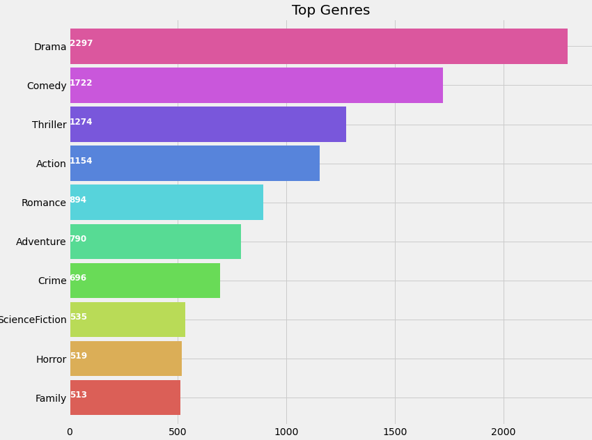

Now let's generate a list ‘genreList’ with all possible unique genres mentioned in the dataset.

現在，我們生成一個列表“ genreList”，其中包含數據集中提到的所有可能的唯一類型。

genreList = []
for index, row in movies.iterrows():
    genres = row["genres"]
    
    for genre in genres:
        if genre not in genreList:
            genreList.append(genre)
genreList[:10] #now we have a list with unique genres

One Hot Encoding for multiple labels

一熱編碼多個標簽

‘genreList’ will now hold all the genres. But how do we come to know about the genres each movie falls into. Now some movies will be ‘Action’, some will be ‘Action, Adventure’, etc. We need to classify the movies according to their genres.

現在，“ genreList”將保留所有類型。 但是我們如何了解每部電影的流派。 現在，有些電影將是“動作”，某些電影將是“動作，冒險”等。我們需要根據電影的類型對電影進行分類。

Let's create a new column in the dataframe that will hold the binary values whether a genre is present or not in it. First let's create a method which will return back a list of binary values for the genres of each movie. The ‘genreList’ will be useful now to compare against the values.

讓我們在數據框中創建一個新列，該列將保存二進制值，無論其中是否存在流派。 首先讓我們創建一個方法，該方法將返回每個電影類型的二進制值列表。 現在，“ genreList”可用于與這些值進行比較。

Let's say for example we have 20 unique genres in the list. Thus the below function will return a list with 20 elements, which will be either 0 or 1. Now for example we have a Movie which has genre = ‘Action’, then the new column will hold [1,0,0,0,0,0,0,0,0,0,0,0,0,0,0,0,0,0,0,0].

舉例來說，清單中有20種獨特的流派。 因此，下面的函數將返回包含20個元素的列表，這些元素將為0或1。現在，例如，我們有一個流派='動作'的電影，那么新列將包含[1,0,0,0， 0,0,0,0,0,0,0,0,0,0,0,0,0,0,0,0]。

Similarly for ‘Action, Adventure’ we will have, [1,1,0,0,0,0,0,0,0,0,0,0,0,0,0,0,0,0,0,0]. Converting the genres into such a list of binary values will help in easily classifying the movies by their genres.

同樣，對于“動作，冒險”，我們將有[1,1,0,0,0,0,0,0,0,0,0,0,0,0,0,0,0,0,0,0 0]。 將流派轉換為這樣的二進制值列表將有助于輕松按電影的流派對電影進行分類。

def binary(genre_list):
    binaryList = []
    
    for genre in genreList:
        if genre in genre_list:
            binaryList.append(1)
        else:
            binaryList.append(0)
    
    return binaryList

Applying the binary() function to the ‘genres’ column to get ‘genre_list’

將binary()函數應用于“類型”列以獲取“ genre_list”

We will follow the same notations for other features like the cast, director, and the keywords.

對于其他功能(例如演員，導演和關鍵字)，我們將使用相同的符號。

movies['genres_bin'] = movies['genres'].apply(lambda x: binary(x))
movies['genres_bin'].head()

第5步-使用Cast列 (Step 5 — Working with the Cast column)

Let’s plot a graph of Actors with Highest Appearances

讓我們繪制出外觀最高的演員圖

plt.subplots(figsize=(12,10))
list1=[]
for i in movies['cast']:
    list1.extend(i)
ax=pd.Series(list1).value_counts()[:15].sort_values(ascending=True).plot.barh(width=0.9,color=sns.color_palette('muted',40))
for i, v in enumerate(pd.Series(list1).value_counts()[:15].sort_values(ascending=True).values): 
    ax.text(.8, i, v,fontsize=10,color='white',weight='bold')
plt.title('Actors with highest appearance')
plt.show()

S

小號

When I initially created the list of all the cast, it had around 50k unique values, as many movies have entries for about 15–20 actors. But do we need all of them? The answer is No. We just need the actors who have the highest contribution to the movie. For eg: The Dark Knight franchise has many actors involved in the movie. But we will select only the main actors like Christian Bale, Micheal Caine, Heath Ledger. I have selected the main 4 actors from each movie.

最初創建所有演員表的列表時，它具有約50k的唯一值，因為許多電影都包含約15–20個演員的條目。 但是我們需要所有這些嗎？ 答案是否定的。我們只需要對電影貢獻最大的演員即可。 例如：黑暗騎士專營權有很多演員都參與了電影。 但我們只會選擇主要演員，例如克里斯蒂安·貝爾，米歇爾·凱恩，希思·萊杰。 我從每部電影中選擇了主要的4位演員。

One question that may arise in your mind is that how do you determine the importance of the actor in the movie. Luckily, the sequence of the actors in the JSON format is according to the actor’s contribution to the movie.

您可能會想到的一個問題是，您如何確定演員在電影中的重要性。 幸運的是，演員的JSON格式順序取決于演員對電影的貢獻。

Let’s see how we do that and create a column ‘cast_bin’

讓我們看看我們如何做到這一點并創建一列' cast_bin '

for i,j in zip(movies['cast'],movies.index):
    list2 = []
    list2 = i[:4]
    movies.loc[j,'cast'] = str(list2)
movies['cast'] = movies['cast'].str.strip('[]').str.replace(' ','').str.replace("'",'')
movies['cast'] = movies['cast'].str.split(',')
for i,j in zip(movies['cast'],movies.index):
    list2 = []
    list2 = i
    list2.sort()
    movies.loc[j,'cast'] = str(list2)
movies['cast']=movies['cast'].str.strip('[]').str.replace(' ','').str.replace("'",'')castList = []
for index, row in movies.iterrows():
    cast = row["cast"]
    
    for i in cast:
        if i not in castList:
            castList.append(i)movies[‘cast_bin’] = movies[‘cast’].apply(lambda x: binary(x))
movies[‘cast_bin’].head()

第6步-使用Directors列 (Step 6 — Working with the Directors column)

Let’s plot Directors with maximum movies

讓我們為導演繪制最多電影

def xstr(s):
    if s is None:
        return ''
    return str(s)
movies['director'] = movies['director'].apply(xstr)plt.subplots(figsize=(12,10))
ax = movies[movies['director']!=''].director.value_counts()[:10].sort_values(ascending=True).plot.barh(width=0.9,color=sns.color_palette('muted',40))
for i, v in enumerate(movies[movies['director']!=''].director.value_counts()[:10].sort_values(ascending=True).values): 
    ax.text(.5, i, v,fontsize=12,color='white',weight='bold')
plt.title('Directors with highest movies')
plt.show()

We create a new column ‘director_bin’ like we have done earlier

我們像之前所做的那樣創建一個新列' director_bin '

directorList=[]
for i in movies['director']:
    if i not in directorList:
        directorList.append(i)movies['director_bin'] = movies['director'].apply(lambda x: binary(x))
movies.head()

So finally, after all this work we get the movies dataset as follows

最后，在完成所有這些工作之后，我們得到了電影數據集，如下所示

第7步-使用“關鍵字”列 (Step 7 — Working with the Keywords column)

The keywords or tags contain a lot of information about the movie, and it is a key feature in finding similar movies. For eg: Movies like “Avengers” and “Ant-man” may have common keywords like superheroes or Marvel.

關鍵字或標簽包含有關電影的大量信息，這是查找相似電影的關鍵功能。 例如：“復仇者聯盟”和“螞蟻俠”之類的電影可能具有超級英雄或漫威等常見關鍵字。

For analyzing keywords, we will try something different and plot a word cloud to get a better intuition:

為了分析關鍵字，我們將嘗試一些不同的方法并繪制詞云以獲得更好的直覺：

from wordcloud import WordCloud, STOPWORDS
import nltk
from nltk.corpus import stopwordsplt.subplots(figsize=(12,12))
stop_words = set(stopwords.words('english'))
stop_words.update(',',';','!','?','.','(',')','$','#','+',':','...',' ','')words=movies['keywords'].dropna().apply(nltk.word_tokenize)
word=[]
for i in words:
    word.extend(i)
word=pd.Series(word)
word=([i for i in word.str.lower() if i not in stop_words])
wc = WordCloud(background_color="black", max_words=2000, stopwords=STOPWORDS, max_font_size= 60,width=1000,height=1000)
wc.generate(" ".join(word))
plt.imshow(wc)
plt.axis('off')
fig=plt.gcf()
fig.set_size_inches(10,10)
plt.show()

We find ‘words_bin’ from Keywords as follows —

我們從關鍵字中找到“ words_bin ”，如下所示-

movies['keywords'] = movies['keywords'].str.strip('[]').str.replace(' ','').str.replace("'",'').str.replace('"','')
movies['keywords'] = movies['keywords'].str.split(',')
for i,j in zip(movies['keywords'],movies.index):
    list2 = []
    list2 = i
    movies.loc[j,'keywords'] = str(list2)
movies['keywords'] = movies['keywords'].str.strip('[]').str.replace(' ','').str.replace("'",'')
movies['keywords'] = movies['keywords'].str.split(',')
for i,j in zip(movies['keywords'],movies.index):
    list2 = []
    list2 = i
    list2.sort()
    movies.loc[j,'keywords'] = str(list2)
movies['keywords'] = movies['keywords'].str.strip('[]').str.replace(' ','').str.replace("'",'')
movies['keywords'] = movies['keywords'].str.split(',')words_list = []
for index, row in movies.iterrows():
    genres = row["keywords"]
    
    for genre in genres:
        if genre not in words_list:
            words_list.append(genre)movies['words_bin'] = movies['keywords'].apply(lambda x: binary(x))
movies = movies[(movies['vote_average']!=0)] #removing the movies with 0 score and without drector names 
movies = movies[movies['director']!='']

步驟8 —電影之間的相似性 (Step 8 — Similarity between movies)

We will be using Cosine Similarity for finding the similarity between 2 movies. How does cosine similarity work?

我們將使用余弦相似度來查找2部電影之間的相似度。 余弦相似度如何工作？

Let’s say we have 2 vectors. If the vectors are close to parallel, i.e. angle between the vectors is 0, then we can say that both of them are “similar”, as cos(0)=1. Whereas if the vectors are orthogonal, then we can say that they are independent or NOT “similar”, as cos(90)=0.

假設我們有2個向量。 如果向量接近平行，即向量之間的夾角為0，則可以說它們都是“相似的”，因為cos(0)= 1。 而如果向量是正交的，那么我們可以說它們是獨立的或不“相似”，因為cos(90)= 0。

For a more detailed study, follow this link.

有關更詳細的研究，請單擊此鏈接 。

Below I have defined a function Similarity, which will check the similarity between the movies.

在下面，我定義了一個相似性功能，該功能將檢查電影之間的相似性。

from scipy import spatialdef Similarity(movieId1, movieId2):
    a = movies.iloc[movieId1]
    b = movies.iloc[movieId2]
    
    genresA = a['genres_bin']
    genresB = b['genres_bin']
    
    genreDistance = spatial.distance.cosine(genresA, genresB)
    
    scoreA = a['cast_bin']
    scoreB = b['cast_bin']
    scoreDistance = spatial.distance.cosine(scoreA, scoreB)
    
    directA = a['director_bin']
    directB = b['director_bin']
    directDistance = spatial.distance.cosine(directA, directB)
    
    wordsA = a['words_bin']
    wordsB = b['words_bin']
    wordsDistance = spatial.distance.cosine(directA, directB)
    return genreDistance + directDistance + scoreDistance + wordsDistance

Let’s check the Similarity between 2 random movies

讓我們檢查兩部隨機電影之間的相似性

We see that the distance is about 2.068, which is high. The more the distance, the less similar the movies are. Let’s see what these random movies actually were.

我們看到該距離約為2.068，這是很高的。 距離越遠，電影越不相似。 讓我們看看這些隨機電影實際上是什么。

It is evident that The Dark Knight Rises and How to train your Dragon 2 are very different movies. Thus the distance is huge.

顯然，《黑暗騎士崛起》和《馴龍高手2》是非常不同的電影。 因此距離很大。

第9步-得分預測器(最后一步！) (Step 9 — Score Predictor (the final step!))

So now when we have everything in place, we will now build the score predictor. The main function working under the hood will be the Similarity() function, which will calculate the similarity between movies, and will find 10 most similar movies. These 10 movies will help in predicting the score for our desired movie. We will take the average of the scores of similar movies and find the score for the desired movie.

因此，當我們準備就緒時，我們現在將建立得分預測器。 幕后工作的主要功能是“ 相似性”函數，該函數將計算電影之間的相似度，并找到10個最相似的電影。 這10部電影將有助于預測我們所需電影的得分。 我們將取相似電影的平均得分，然后找到所需電影的得分。

Now the similarity between the movies will depend on our newly created columns containing binary lists. We know that features like the director or the cast will play a very important role in the movie’s success. We always assume that movies from David Fincher or Chris Nolan will fare very well. Also if they work with their favorite actors, who always fetch them success and also work on their favorite genres, then the chances of success are even higher. Using these phenomena, let's try building our score predictor.

現在，電影之間的相似性將取決于我們新創建的包含二進制列表的列。 我們知道導演或演員等功能將在電影的成功中扮演非常重要的角色。 我們始終認為，大衛·芬奇(David Fincher)或克里斯·諾蘭(Chris Nolan)的電影會很不錯。 同樣，如果他們與自己喜歡的演員合作，他們總是獲得成功，并且也按照自己喜歡的類型工作，那么成功的機會就更高。 利用這些現象，讓我們嘗試構建分數預測器。

import operatordef predict_score():
    name = input('Enter a movie title: ')
    new_movie = movies[movies['original_title'].str.contains(name)].iloc[0].to_frame().T
    print('Selected Movie: ',new_movie.original_title.values[0])
    def getNeighbors(baseMovie, K):
        distances = []
    
        for index, movie in movies.iterrows():
            if movie['new_id'] != baseMovie['new_id'].values[0]:
                dist = Similarity(baseMovie['new_id'].values[0], movie['new_id'])
                distances.append((movie['new_id'], dist))
    
        distances.sort(key=operator.itemgetter(1))
        neighbors = []
    
        for x in range(K):
            neighbors.append(distances[x])
        return neighbors
    
    K = 10
    avgRating = 0
    neighbors = getNeighbors(new_movie, K)print('\nRecommended Movies: \n')
    for neighbor in neighbors:
        avgRating = avgRating+movies.iloc[neighbor[0]][2]  
        print( movies.iloc[neighbor[0]][0]+" | Genres: "+str(movies.iloc[neighbor[0]][1]).strip('[]').replace(' ','')+" | Rating: "+str(movies.iloc[neighbor[0]][2]))
    
    print('\n')
    avgRating = avgRating/K
    print('The predicted rating for %s is: %f' %(new_movie['original_title'].values[0],avgRating))
    print('The actual rating for %s is %f' %(new_movie['original_title'].values[0],new_movie['vote_average']))

Now simply just run the function as follows and enter the movie you like to find 10 similar movies and it’s predicted ratings

現在，只需按如下所示運行該功能，然后輸入您想要的電影，即可找到10部相似的電影及其預測的收視率

predict_score()

Thus we have completed the Movie Recommendation System implementation using the K Nearest Neighbors algorithm.

因此，我們已經使用K最近鄰算法完成了電影推薦系統的實現。

旁注— K值 (Sidenote — K Value)

In this project, I have arbitrarily chosen the value K=10.

在這個項目中，我任意選擇了值K = 10。

But in other applications of KNN, finding the value of K is not easy. A small value of K means that noise will have a higher influence on the result and a large value make it computationally expensive. Data scientists usually choose as an odd number if the number of classes is 2 and another simple approach to select k is set K=sqrt(n).

但是在KNN的其他應用中，找到K的值并不容易。 較小的K值意味著噪聲將對結果產生更大的影響，而較大的值將使其在計算上昂貴。 如果類別數是2，并且選擇k的另一種簡單方法是K = sqrt(n)，則數據科學家通常選擇作為奇數。

This is the end of this blog. Let me know if you have any suggestions/doubts.

這是本博客的結尾。 如果您有任何建議/疑問，請告訴我。

Find the Python notebook with the entire code along with the dataset and all the illustrations here.Let me know how you found this blog :)

在 此處 找到帶有完整代碼以及數據集和所有插圖的Python筆記本 。讓我知道您如何找到此博客：)

進一步閱讀 (Further Reading)

1. Recommender System

   推薦系統

2. Machine Learning Basics with the K-Nearest Neighbors Algorithm

   使用K最近鄰算法的機器學習基礎

3. Recommender Systems with Python — Part II: Collaborative Filtering (K-Nearest Neighbors Algorithm)

   使用Python的推薦系統—第二部分：協同過濾(K最近鄰算法)

4. What is Cosine Similarity?

   什么是余弦相似度？

5. How to find the optimal value of K in KNN?

   如何在KNN中找到K的最優值？