In this article, we will go through the end-to-end pipeline of training convolution neural networks, i.e. organizing the data into directories, preprocessing, data augmentation, model building, etc.

在本文中，我們將遍歷訓練卷積神經網絡的端到端管道，即將數據組織到目錄，預處理，數據擴充，模型構建等中。

We will spend a good amount of time on data preprocessing techniques commonly used with image processing. This is because preprocessing takes about 50–80% of your time in most deep learning projects, and knowing some useful tricks will help you a lot in your projects. We will be using the flowers dataset from Kaggle to demonstrate the key concepts. To get into the codes directly, an accompanying notebook is published on Kaggle(Please use a CPU for running the initial parts of the code and GPU for model training).

我們將在圖像處理常用的數據預處理技術上花費大量時間。 這是因為在大多數深度學習項目中，預處理需要花費您大約50-80％的時間，并且了解一些有用的技巧將對您的項目有很大幫助。 我們將使用來自Kaggle的flowers數據集來演示關鍵概念。 為了直接進入代碼，在Kaggle上發布了一個附帶的筆記本 (請使用CPU運行代碼的初始部分，并使用GPU進行模型訓練)。

導入數據集 (Importing the dataset)

Let’s begin with importing the necessary libraries and loading the dataset. This is a requisite step in every data analysis process.

讓我們從導入必要的庫并加載數據集開始。 這是每個數據分析過程中的必要步驟。

# Importing necessary librariesimport keras
import tensorflow
from skimage import io
import os
import glob
import numpy as np
import random
import matplotlib.pyplot as plt
%matplotlib inline# Importing and Loading the data into data frame
#class 1 - Rose, class 0- DaisyDATASET_PATH = '../input/flowers-recognition/flowers/'
flowers_cls = ['daisy', 'rose']# glob through the directory (returns a list of all file paths)flower_path = os.path.join(DATASET_PATH, flowers_cls[1], '*')
flower_path = glob.glob(flower_path)# access some element (a file) from the list
image = io.imread(flower_path[251])

數據預處理 (Data Preprocessing)

圖片-頻道和大小 (Images — Channels and Sizes)

Images come in different shapes and sizes. They also come through different sources. For example, some images are what we call “natural images”, which means they are taken in color, in the real world. For example:

圖像具有不同的形狀和大小。 它們也來自不同的來源 。 例如，有些圖像被我們稱為“自然圖像”，這意味著它們是在現實世界中以彩色拍攝的。 例如：

• A picture of a flower is a natural image.
  花的圖片是自然圖像。

• An X-ray image is not a natural image.

  X射線圖像不是自然圖像。

Taking all these variations into consideration, we need to perform some pre-processing on any image data. RGB is the most popular encoding format, and most “natural images” we encounter are in RGB. Also, among the first step of data pre-processing is to make the images of the same size. Let’s move on to how we can change the shape and form of images.

考慮到所有這些變化，我們需要對任何圖像數據進行一些預處理。 RGB是最流行的編碼格式，我們遇到的大多數“自然圖像”都是RGB。 同樣，數據預處理的第一步是使圖像大小相同。 讓我們繼續介紹如何更改圖像的形狀和形式。

# plotting the original image and the RGB channels
f, (ax1, ax2, ax3, ax4) = plt.subplots(1, 4, sharey=True)
f.set_figwidth(15)
ax1.imshow(image)# RGB channels
# CHANNELID : 0 for Red, 1 for Green, 2 for Blue. 
ax2.imshow(image[:, : , 0]) #Red
ax3.imshow(image[:, : , 1]) #Green
ax4.imshow(image[:, : , 2]) #Blue
f.suptitle('Different Channels of Image')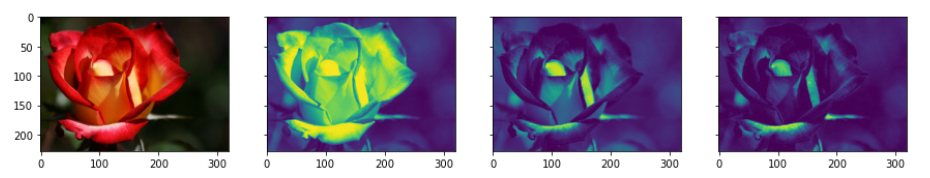

形態轉換 (Morphological Transformations)

The term morphological transformation refers to any modification involving the shape and form of the images. These are very often used in image analysis tasks. Although they are used with all types of images, they are especially powerful for images that are not natural (come from a source other than a picture of the real world). The typical transformations are erosion, dilation, opening, and closing. Let’s now look at some code to implement these morphological transformations.

術語形態變換是指涉及圖像形狀和形式的任何修飾。 這些通常在圖像分析任務中使用。 盡管它們可用于所有類型的圖像，但對于非自然的圖像(來自真實世界的圖片以外的其他來源)，它們尤其強大。 典型的轉換是侵蝕，膨脹，打開和關閉。 現在讓我們看一些實現這些形態轉換的代碼。

1.Thresholding

1.閾值

One of the simpler operations where we take all the pixels whose intensities are above a certain threshold and convert them to ones; the pixels having value less than the threshold are converted to zero. This results in a binary image.

一種比較簡單的操作，其中我們將強度高于特定閾值的所有像素都轉換為像素； 值小于閾值的像素將轉換為零。 這將產生二進制圖像 。

# bin_image will be a (240, 320) True/False array
#The range of pixel varies between 0 to 255
#The pixel having black is more close to 0 and pixel which is white is more close to 255
# 125 is Arbitrary heuristic measure halfway between 1 and 255 (the range of image pixel) 
bin_image = image[:, :, 0] > 125
plot_image([image, bin_image], cmap='gray')

2.Erosion, Dilation, Opening & Closing

2.侵蝕，膨脹，開合

Erosion shrinks bright regions and enlarges dark regions. Dilation on the other hand is exact opposite side — it shrinks dark regions and enlarges the bright regions.

侵蝕使明亮的區域收縮，使黑暗的區域擴大。 另一方面， 膨脹恰好在相反的一面-它會縮小深色區域并擴大明亮區域。

Opening is erosion followed by dilation. Opening can remove small bright spots (i.e. “salt”) and connect small dark cracks. This tends to “open” up (dark) gaps between (bright) features.

開放是侵蝕，然后是膨脹。 開口可以去除小的亮點(即“鹽”)并連接小的暗裂紋。 這往往會“打開”(亮)特征之間的(暗)間隙。

Closing is dilation followed by erosion. Closing can remove small dark spots (i.e. “pepper”) and connect small bright cracks. This tends to “close” up (dark) gaps between (bright) features.

關閉是擴張，然后是侵蝕。 關閉可以消除小黑點(即“胡椒”)并連接小亮點。 這往往會“縮小”(亮)特征之間的(暗)間隙。

All these can be done using the skimage.morphology module. The basic idea is to have a circular disk of a certain size (3 below) move around the image and apply these transformations using it.

所有這些都可以使用skimage.morphology模塊完成。 基本思想是讓一定大小(以下為3)的圓盤在圖像周圍移動并使用該圖像應用這些轉換。

from skimage.morphology import binary_closing, binary_dilation, binary_erosion, binary_opening
from skimage.morphology import selem# use a disk of radius 3
selem = selem.disk(3)# oprning and closing
open_img = binary_opening(bin_image, selem)
close_img = binary_closing(bin_image, selem)
# erosion and dilation
eroded_img = binary_erosion(bin_image, selem)
dilated_img = binary_dilation(bin_image, selem)
plot_image([bin_image, open_img, close_img, eroded_img, dilated_img], cmap='gray')

正常化 (Normalisation)

Normalisation is the most crucial step in the pre-processing part. This refers to rescaling the pixel values so that they lie within a confined range. One of the reasons to do this is to help with the issue of propagating gradients. There are multiple ways to normalize images that we will be talking about.

標準化是預處理部分中最關鍵的步驟。 這是指重新縮放像素值，以使其位于限定范圍內。 這樣做的原因之一是幫助解決傳播梯度的問題。 我們將討論多種標準化圖像的方法。

#way1-this is common technique followed in case of RGB images 
norm1_image = image/255#way2-in case of medical Images/non natural images 
norm2_image = image - np.min(image)/np.max(image) - np.min(image)#way3-in case of medical Images/non natural images 
norm3_image = image - np.percentile(image,5)/ np.percentile(image,95) - np.percentile(image,5)
plot_image([image, norm1_image, norm2_image, norm3_image], cmap='gray')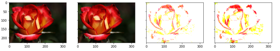

增廣 (Augmentation)

This brings us to the next aspect of data pre-processing — data augmentation. Many times, the quantity of data that we have is not sufficient to perform the task of classification well enough. In such cases, we perform data augmentation. As an example, if we are working with a dataset of classifying gemstones into their different types, we may not have enough number of images (since high-quality images are difficult to obtain). In this case, we can perform augmentation to increase the size of your dataset. Augmentation is often used in image-based deep learning tasks to increase the amount and variance of training data. Augmentation should only be done on the training set, never on the validation set.

這使我們進入了數據預處理的下一個方面-數據增強。 很多時候， 我們擁有的數據量不足以充分執行分類任務。 在這種情況下，我們將執行數據擴充 。 例如，如果我們正在使用將寶石分類為不同類型的數據集，則可能沒有足夠數量的圖像(因為很難獲得高質量的圖像)。 在這種情況下，我們可以執行擴充以增加數據集的大小。 增強通常用于基于圖像的深度學習任務中，以增加訓練數據的數量和方差。 增強只能在訓練集上進行，而不能在驗證集上進行。

As you know that pooling increases the invariance. If a picture of a dog is in the top left corner of an image, with pooling, you would be able to recognize if the dog is in little bit left/right/up/down around the top left corner. But with training data consisting of data augmentation like flipping, rotation, cropping, translation, illumination, scaling, adding noise, etc., the model learns all these variations. This significantly boosts the accuracy of the model. So, even if the dog is there at any corner of the image, the model will be able to recognize it with high accuracy.

如您所知， 合并會增加不變性。 如果狗的圖片位于圖像的左上角，則通過合并，您將能夠識別出狗是否在左上角的左/右/上/下一點點。 但是，通過包含翻轉，旋轉，裁剪，平移，照度，縮放，添加噪聲等數據增強的訓練數據，該模型可以學習所有這些變化。 這大大提高了模型的準確性。 因此，即使狗在圖像的任何角落，模型也將能夠高精度地識別它。

There are multiple types of augmentations possible. The basic ones transform the original image using one of the following types of transformations:

可能有多種類型的擴充。 基本的使用以下類型的轉換之一來轉換原始圖像：

1. Linear transformations
   線性變換
2. Affine transformations
   仿射變換

from skimage import transform as tf
# flip left-right, up-down
image_flipr = np.fliplr(image)
image_flipud = np.flipud(image)
plot_image([image, image_flipr, image_flipud])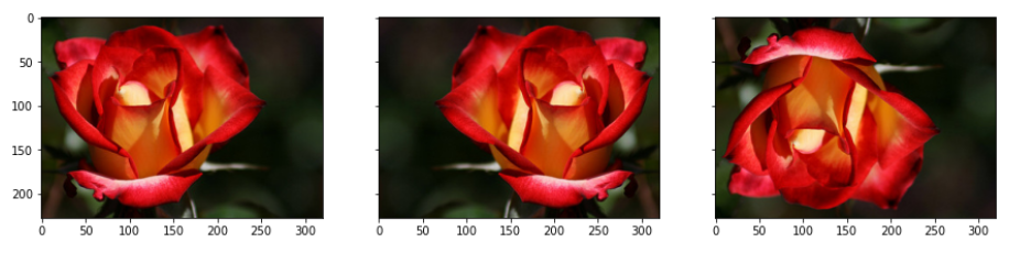

# specify x and y coordinates to be used for shifting (mid points)
shift_x, shift_y = image.shape[0]/2, image.shape[1]/2# translation by certain units
matrix_to_topleft = tf.SimilarityTransform(translation=[-shift_x, -shift_y])
matrix_to_center = tf.SimilarityTransform(translation=[shift_x, shift_y])# rotation
rot_transforms =  tf.AffineTransform(rotation=np.deg2rad(45))
rot_matrix = matrix_to_topleft + rot_transforms + matrix_to_center
rot_image = tf.warp(image, rot_matrix)# scaling 
scale_transforms = tf.AffineTransform(scale=(2, 2))
scale_matrix = matrix_to_topleft + scale_transforms + matrix_to_center
scale_image_zoom_out = tf.warp(image, scale_matrix)
scale_transforms = tf.AffineTransform(scale=(0.5, 0.5))
scale_matrix = matrix_to_topleft + scale_transforms + matrix_to_center
scale_image_zoom_in = tf.warp(image, scale_matrix)# translation
transaltion_transforms = tf.AffineTransform(translation=(50, 50))
translated_image = tf.warp(image, transaltion_transforms)
plot_image([image, rot_image, scale_image_zoom_out, scale_image_zoom_in, translated_image])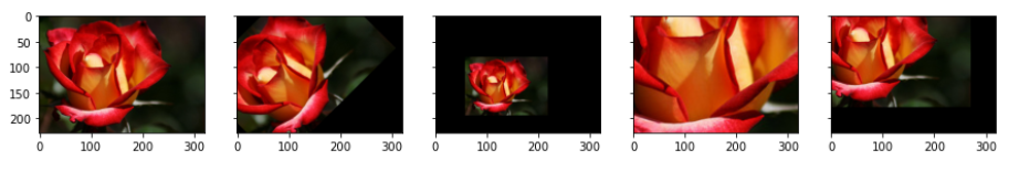

# shear transforms
shear_transforms = tf.AffineTransform(shear=np.deg2rad(45))
shear_matrix = matrix_to_topleft + shear_transforms + matrix_to_center
shear_image = tf.warp(image, shear_matrix)
bright_jitter = image*0.999 + np.zeros_like(image)*0.001
plot_image([image, shear_image, bright_jitter])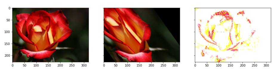

網絡建設 (Network Building)

Let’s now build and train the model.

現在讓我們構建和訓練模型。

選擇架構 (Choosing the architecture)

We will use ‘ResNet’ architecture in this section. Since ResNets have become quite prevalent in the industry, it is worth spending some time to understand the important elements of their architecture. Let’s start with the original architecture proposed here. Also, in 2016, the ResNet team had proposed some improvements in the original architecture here. Using these modifications, they had trained nets of more than 1000 layers (e.g. ResNet-1001).

在本節中，我們將使用“ ResNet ”架構。 由于ResNets在行業中已變得相當普遍，因此值得花一些時間來了解其體系結構的重要元素。 讓我們從這里提出的原始架構開始 。 此外，在2016年，RESNET隊曾提議在原有的架構有所改善這里 。 使用這些修改，他們訓練了超過1000層的網絡 (例如ResNet-1001 )。

The ‘ResNet builder’ module which is used here is basically a Python module containing all the building blocks of ResNet. We will use this module to import the variants of ResNets (ResNet-18, ResNet-34, etc.). The resnet.py module is taken from here. Its biggest upside is that the ‘skip connections’ mechanism allows very deep networks.

這里使用的“ ResNet builder”模塊基本上是一個Python模塊，其中包含ResNet的所有構建塊。 我們將使用此模塊導入ResNet的變體(ResNet-18，ResNet-34等)。 resnet.py模塊來自此處 。 其最大的好處是“跳過連接”機制允許非常深的網絡。

運行數據生成器 (Run a data generator)

Data generator supports preprocessing — it normalizes the images (dividing by 255) and crops the center (100 x 100) portion of the image.

數據生成器支持預處理-標準化圖像(除以255)并裁剪圖像的中心(100 x 100)部分。

There was no specific reason to include 100 as the dimension but it has been chosen so that we can process all the images which are of greater than 100*100 dimension. If any dimension (height or width) of an image is less than 100 pixels, then that image is deleted automatically. You can change it to 150 or 200 according to your need.

沒有特別的理由將100作為尺寸，但是選擇它是為了我們可以處理所有尺寸大于100 * 100的圖像。 如果圖像的任何尺寸(高度或寬度)小于100像素，則該圖像將被自動刪除。 您可以根據需要將其更改為150或200。

Let’s now set up the data generator. The code below sets up a custom data generator which is slightly different than the one that comes with the keras API. The reason to use a custom generator is to be able to modify it according to the problem at hand (customizability).

現在設置數據生成器 。 下面的代碼設置了一個自定義數據生成器，該數據生成器與keras API附帶的自定義數據生成器略有不同。 使用定制生成器的原因是能夠根據當前問題(可定制性)對其進行修改。

import numpy as np
import keras
class DataGenerator(keras.utils.Sequence):
    'Generates data for Keras'
    
    def __init__(self, mode='train', ablation=None, flowers_cls=['daisy', 'rose'], 
                 batch_size=32, dim=(100, 100), n_channels=3, shuffle=True):
        """
        Initialise the data generator
        """
        self.dim = dim
        self.batch_size = batch_size
        self.labels = {}
        self.list_IDs = []
        
        # glob through directory of each class 
        for i, cls in enumerate(flowers_cls):
            paths = glob.glob(os.path.join(DATASET_PATH, cls, '*'))
            brk_point = int(len(paths)*0.8)
            if mode == 'train':
                paths = paths[:brk_point]
            else:
                paths = paths[brk_point:]
            if ablation is not None:
                paths = paths[:ablation]
            self.list_IDs += paths
            self.labels.update({p:i for p in paths})
            
        self.n_channels = n_channels
        self.n_classes = len(flowers_cls)
        self.shuffle = shuffle
        self.on_epoch_end()
    def __len__(self):
        'Denotes the number of batches per epoch'
        return int(np.floor(len(self.list_IDs) / self.batch_size))
    def __getitem__(self, index):
        'Generate one batch of data'
        # Generate indexes of the batch
        indexes = self.indexes[index*self.batch_size:(index+1)*self.batch_size]
        # Find list of IDs
        list_IDs_temp = [self.list_IDs[k] for k in indexes]
        # Generate data
        X, y = self.__data_generation(list_IDs_temp)
        return X, y
    def on_epoch_end(self):
        'Updates indexes after each epoch'
        self.indexes = np.arange(len(self.list_IDs))
        if self.shuffle == True:
            np.random.shuffle(self.indexes)
    def __data_generation(self, list_IDs_temp):
        'Generates data containing batch_size samples' # X : (n_samples, *dim, n_channels)
        # Initialization
        X = np.empty((self.batch_size, *self.dim, self.n_channels))
        y = np.empty((self.batch_size), dtype=int)
        
        delete_rows = []
        # Generate data
        for i, ID in enumerate(list_IDs_temp):
            # Store sample
            img = io.imread(ID)
            img = img/255
            if img.shape[0] > 100 and img.shape[1] > 100:
                h, w, _ = img.shape
                img = img[int(h/2)-50:int(h/2)+50, int(w/2)-50:int(w/2)+50, : ]
            else:
                delete_rows.append(i)
                continue
            
            X[i,] = img
          
            # Store class
            y[i] = self.labels[ID]
        
        X = np.delete(X, delete_rows, axis=0)
        y = np.delete(y, delete_rows, axis=0)
        return X, keras.utils.to_categorical(y, num_classes=self.n_classes)

To start with, we have the training data stored in nn directories (if there are nn classes). For a given batch size, we want to generate batches of data points and feed them to the model.

首先，我們將訓練數據存儲在nn目錄中(如果有nn個類)。 對于給定的批處理大小，我們希望生成一批數據點并將其饋送到模型中。

The first for loop 'globs' through each of the classes (directories). For each class, it stores the path of each image in the list paths. In training mode, it subsets paths to contain the first 80% images; in validation mode it subsets the last 20%. In the special case of an ablation experiment, it simply subsets the first ablation images of each class.

每個類(目錄)的第一個for循環“全局對象”。 對于每個類，它將每個圖像的路徑存儲在列表paths 。 在訓練模式下，它對paths進行子集以包含前80％的圖像； 在驗證模式下，它會將最后20％的內容作為子集。 在消融實驗的特殊情況下，它只是將每個類別的第一個ablation圖像進行子集化。

We store the paths of all the images (of all classes) in a combined list self.list_IDs. The dictionary self.labels contains the labels (as key:value pairs of path: class_number (0/1)).

我們將所有圖像(所有類)的路徑存儲在組合列表self.list_IDs 。 字典self.labels包含標簽(作為path: class_number (0/1) key：value對path: class_number (0/1) )。

After the loop, we call the method on_epoch_end(), which creates an array self.indexes of length self.list_IDs and shuffles them (to shuffle all the data points at the end of each epoch).

循環之后，我們調用方法on_epoch_end() ，該方法創建一個長度為self.list_IDs的數組self.list_IDs并self.indexes進行self.list_IDs (以在每個紀元末尾對所有數據點進行self.list_IDs )。

The _getitem_ method uses the (shuffled) array self.indexes to select a batch_size number of entries (paths) from the path list self.list_IDs.

該_getitem_方法使用(洗牌)陣列self.indexes選擇batch_size從路徑列表中的條目(路徑)數self.list_IDs 。

Finally, the method __data_generation returns the batch of images as the pair X, y where X is of shape (batch_size, height, width, channels) and y is of shape (batch size, ). Note that __data_generation also does some preprocessing - it normalises the images (divides by 255) and crops the center 100 x 100 portion of the image. Thus, each image has the shape (100, 100, num_channels). If any dimension (height or width) of an image less than 100 pixels, that image is deleted.

最后，方法__data_generation返回成對的圖像批次X，y，其中X的形狀為(batch_size, height, width, channels)而y的形狀為(batch size, ) 。 請注意， __data_generation還執行一些預處理-將圖像__data_generation (除以255)并__data_generation圖像中心100 x 100。 因此，每個圖像具有形狀(100, 100, num_channels) 。 如果圖像的任何尺寸(高度或寬度)小于100像素，則會刪除該圖像。

消融實驗 (Ablation Experiments)

These refer to taking a small chunk of data and running your model on it — this helps in figuring out if the model is running at all. This is called an ablation experiment.

這些指的是獲取一小部分數據并在其上運行模型-這有助于確定模型是否在運行。 這稱為消融實驗。

The first part of building a network is to get it to run on your dataset. Let’s try fitting the net on only a few images and just one epoch. Note that since ablation=100 is specified, 100 images of each class are used, so total number of batches is np.floor(200/32) = 6.

構建網絡的第一步是使它在數據集上運行。 讓我們嘗試僅在少數幾個圖像和一個紀元上擬合網絡。 請注意，由于指定了ablation=100 ，因此每個類別使用100張圖像，因此批次總數為np.floor(200/32) = 6。

Note that the DataGenerator class 'inherits' from the keras.utils.Sequence class, so it has all the functionalities of the base keras.utils.Sequence class (such as the model.fit_generator method).

注意， DataGenerator從類繼承“ keras.utils.Sequence類，因此它具有基的所有功能keras.utils.Sequence類(如model.fit_generator方法)。

# using resnet 18
model = resnet.ResnetBuilder.build_resnet_18((img_channels, img_rows, img_cols), nb_classes)
model.compile(loss='categorical_crossentropy', optimizer='SGD',
              metrics=['accuracy'])# create data generator objects in train and val mode
# specify ablation=number of data points to train on
training_generator = DataGenerator('train', ablation=100)
validation_generator = DataGenerator('val', ablation=100)# fit: this will fit the net on 'ablation' samples, only 1 epoch
model.fit_generator(generator=training_generator,
                    validation_data=validation_generator,
                    epochs=1,)

過度擬合訓練數據 (Overfitting on Training Data)

The next step is trying to overfit the model on the training data. Why would we want to intentionally overfit on our data? Simply put, this will tell us whether the network is capable of learning the patterns in the training set. This tells you whether the model is behaving as expected or not.

下一步是嘗試對訓練數據過度擬合模型。 我們為什么要故意過度擬合我們的數據？ 簡而言之，這將告訴我們網絡是否能夠學習訓練集中的模式。 這將告訴您模型是否表現出預期的行為。

We’ll use ablation=100 (i.e. training on 100 images of each class), so it is still a very small dataset, and we will use 20 epochs. In each epoch, 200/32=6 batches will be used.

我們將使用ablation = 100(即在每個類上訓練100張圖像)，因此它仍然是一個非常小的數據集，并且將使用20個紀元。 在每個時代，將使用200/32 = 6批。

# resnet 18
model = resnet.ResnetBuilder.build_resnet_18((img_channels, img_rows, img_cols), nb_classes)
model.compile(loss='categorical_crossentropy',optimizer='SGD',
              metrics=['accuracy'])# generators
training_generator = DataGenerator('train', ablation=100)
validation_generator = DataGenerator('val', ablation=100)# fit
model.fit_generator(generator=training_generator,
                    validation_data=validation_generator,
                    epochs=20)

The results show that the training accuracy increases consistently with each epoch. The validation accuracy also increases and then plateaus out — this is a sign of ‘good fit’, i.e. we know that the model is at least able to learn from a small dataset, so we can hope that it will be able to learn from the entire set as well.

結果表明，訓練精度隨著每個時期的增加而一致。 驗證準確性也會提高，然后達到平穩狀態–這是“良好擬合”的標志，即我們知道該模型至少能夠從較小的數據集中學習，因此我們希望它能夠從整套也是如此。

To summarise, a good test of any model is to check whether it can overfit on the training data (i.e. the training loss consistently reduces along epochs). This technique is especially useful in deep learning because most deep learning models are trained on large datasets, and if they are unable to overfit a small version, then they are unlikely to learn from the larger version.

綜上所述，對任何模型的一個很好的測試是檢查它是否可以對訓練數據過度擬合 (即訓練損失沿歷時不斷減少)。 這項技術在深度學習中特別有用，因為大多數深度學習模型都是在大型數據集上進行訓練的，并且如果它們無法適合較小的版本，則他們不太可能從較大的版本中學習。

超參數調整 (Hyperparameter tuning)

we trained the model on a small chunk of the dataset and confirmed that the model can learn from the dataset (indicated by overfitting). After fixing the model and data augmentation, we now need to find the learning rate for the optimizer (here SGD). First, let’s make a list of the hyper-parameters we want to tune:

我們在數據集中的一小部分上對模型進行了訓練，并確認該模型可以從數據集中學習(通過過度擬合表示)。 修正模型和數據擴充之后，我們現在需要找到優化器的學習率(此處為SGD)。 首先，讓我們列出要調整的超參數：

1. Learning Rate & Variation + Optimisers
   學習率與變異+優化器
2. Augmentation Techniques
   增強技術

The basic idea is to track the validation loss with increasing epochs for various values of a hyperparameter.

基本思想是隨著超參數的各種值的增加而跟蹤驗證損失。

Keras Callbacks

Keras回調

Before you move ahead, let’s discuss a bit about callbacks. Callbacks are basically actions that you want to perform at specific instances of training. For example, we want to perform the action of storing the loss at the end of every epoch (the instance here is the end of an epoch).

在繼續之前，讓我們討論一下回調 。 回調基本上是您想要在特定訓練實例上執行的操作。 例如，我們想要執行在每個時期結束時存儲損失的操作(這里的實例是一個時期的結束)。

Formally, a callback is simply a function (if you want to perform a single action), or a list of functions (if you want to perform multiple actions), which are to be executed at specific events (end of an epoch, start of every batch, when the accuracy plateaus out, etc.). Keras provides some very useful callback functionalities through the class keras.callbacks.Callback.

形式上，回調只是一個函數(如果要執行單個動作)或函數列表(如果要執行多個動作)，它們將在特定事件(時期結束，開始時)執行每批，精度達到穩定水平時等)。 keras.callbacks.Callback通過類keras.callbacks.Callback提供了一些非常有用的回調功能。

Keras has many builtin callbacks (listed here). The generic way to create a custom callback in keras is:

Keras有許多內置的回調( 在此處列出 )。 在keras中創建自定義回調的通用方法是：

from keras import optimizers
from keras.callbacks import *# range of learning rates to tune
hyper_parameters_for_lr = [0.1, 0.01, 0.001]# callback to append loss
class LossHistory(keras.callbacks.Callback):
    def on_train_begin(self, logs={}):
        self.losses = []
    def on_epoch_end(self, epoch, logs={}):
        self.losses.append(logs.get('loss'))# instantiate a LossHistory() object to store histories
history = LossHistory()
plot_data = {}# for each hyperparam: train the model and plot loss history
for lr in hyper_parameters_for_lr:
    print ('\n\n'+'=='*20 + '   Checking for LR={}  '.format(lr) + '=='*20 )
    sgd = optimizers.SGD(lr=lr, clipnorm=1.)
        # model and generators
    model = resnet.ResnetBuilder.build_resnet_18((img_channels, img_rows, img_cols), nb_classes)
    model.compile(loss='categorical_crossentropy',optimizer= sgd,
                  metrics=['accuracy'])
    training_generator = DataGenerator('train', ablation=100)
    validation_generator = DataGenerator('val', ablation=100)
    model.fit_generator(generator=training_generator,
                        validation_data=validation_generator,
                        epochs=3, callbacks=[history])
        # plot loss history
    plot_data[lr] = history.losses

In the code above, we have created a custom callback to append the loss to a list at the end of every epoch. Note that logs is an attribute (a dictionary) of keras.callbacks.Callback, and we are using it to get the value of the key 'loss'. Some other keys of this dict are acc, val_loss etc.

在上面的代碼中，我們創建了一個自定義回調，以將損失附加到每個時期末尾的列表中。 請注意， logs是keras.callbacks.Callback的屬性(字典)，我們正在使用它來獲取鍵“ loss”的值。 此字典的其他一些鍵是acc ， val_loss等。

To tell the model that we want to use a callback, we create an object of LossHistory called history and pass it to model.fit_generator using callbacks=[history]. In this case, we only have one callback history, though you can pass multiple callback objects through this list (an example of multiple callbacks is in the section below - see the code block of DecayLR()).

為了告訴模型我們要使用回調，我們創建了一個名為history的LossHistory對象，并使用callbacks=[history]將其傳遞給model.fit_generator 。 在這種情況下，我們只有一個回調history ，盡管您可以通過此列表傳??遞多個回調對象(以下部分中為多個回調的示例-請參見DecayLR()的代碼塊)。

Here, we tuned the learning rate hyperparameter and observed that a rate of 0.1 is the optimal learning rate when compared to 0.01 and 0.001. However, using such a high learning rate for the entire training process is not a good idea since the loss may start to oscillate around the minima later. So, at the start of the training, we use a high learning rate for the model to learn fast, but as we train further and proceed towards the minima, we decrease the learning rate gradually.

在這里， 我們調整了學習率超參數，并觀察到與0.01和0.001相比，0.1是最佳學習率。 但是，在整個訓練過程中使用如此高的學習率并不是一個好主意，因為稍后損失可能會開始圍繞最小值移動。 因此，在訓練開始時，我們使用較高的學習率來使模型快速學習，但是隨著我們進一步訓練并朝著最小值邁進，我們會逐漸降低學習率。

# plot loss history for each value of hyperparameter
f, axes = plt.subplots(1, 3, sharey=True)
f.set_figwidth(15)
plt.setp(axes, xticks=np.arange(0, len(plot_data[0.01]), 1)+1)
for i, lr in enumerate(plot_data.keys()):
    axes[i].plot(np.arange(len(plot_data[lr]))+1, plot_data[lr])

The results above show that a learning rate of 0.1 is the best, though using such a high learning rate for the entire training is usually not a good idea. Thus, we should use learning rate decay — starting from a high learning rate and decaying it with every epoch.

上面的結果表明，學習速度最好為0.1，盡管在整個訓練過程中使用如此高的學習速度通常不是一個好主意。 因此，我們應該使用學習率衰減 -從較高的學習率開始，然后在每個時期都將其衰減。

We use another custom callback (DecayLR) to decay the learning rate at the end of every epoch. The decay rate is specified as 0.5 ^ epoch. Also, note that this time we are telling the model to use two callbacks (passed as a list callbacks=[history, decay] to model.fit_generator).

我們使用另一個自定義回調 ( DecayLR )在每個時期結束時降低學習率。 衰減率指定為0.5 ^ epoch。 另外，請注意，這次我們告訴模型使用兩個回調 (作為列表callbacks=[history, decay]傳遞給model.fit_generator callbacks=[history, decay] )。

Although we have used our own custom decay implementation here, you can use the ones built into keras optimisers (using the decay argument).

盡管我們在這里使用了自己的自定義衰減實現，但是您可以使用內置在keras優化器中的實現 (使用decay參數)。

# learning rate decay
class DecayLR(keras.callbacks.Callback):
    def __init__(self, base_lr=0.001, decay_epoch=1):
        super(DecayLR, self).__init__()
        self.base_lr = base_lr
        self.decay_epoch = decay_epoch 
        self.lr_history = []
        
    # set lr on_train_begin
    def on_train_begin(self, logs={}):
        K.set_value(self.model.optimizer.lr, self.base_lr)    # change learning rate at the end of epoch
    def on_epoch_end(self, epoch, logs={}):
        new_lr = self.base_lr * (0.5 ** (epoch // self.decay_epoch))
        self.lr_history.append(K.get_value(self.model.optimizer.lr))
        K.set_value(self.model.optimizer.lr, new_lr)# to store loss history
history = LossHistory()
plot_data = {}# start with lr=0.1
decay = DecayLR(base_lr=0.1)# model
sgd = optimizers.SGD()
model = resnet.ResnetBuilder.build_resnet_18((img_channels, img_rows, img_cols), nb_classes)
model.compile(loss='categorical_crossentropy',optimizer= sgd,
              metrics=['accuracy'])
training_generator = DataGenerator('train', ablation=100)
validation_generator = DataGenerator('val', ablation=100)
model.fit_generator(generator=training_generator,
                    validation_data=validation_generator,
                    epochs=3, callbacks=[history, decay])
plot_data[lr] = decay.lr_history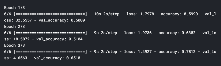

plt.plot(np.arange(len(decay.lr_history)), decay.lr_history)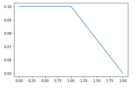

Augmentation Techniques

增強技術

Let’s now write some code to implement data augmentation. Augmentation is usually done with data generators, i.e. the augmented data is generated batch-wise, on the fly. You can either use the built-in keras ImageDataGenerator or write your own data generator (for some custom features etc if you want). The below code show how to implement these.

現在讓我們編寫一些代碼來實現數據擴充。 增強通常是通過數據生成器完成的，即增強的數據是動態地分批生成的。 您可以使用內置的keras ImageDataGenerator或編寫自己的數據生成器(如果需要，可以使用某些自定義功能等)。 下面的代碼顯示了如何實現這些。

import numpy as np
import keras# data generator with augmentation
class AugmentedDataGenerator(keras.utils.Sequence):
    'Generates data for Keras'
    def __init__(self, mode='train', ablation=None, flowers_cls=['daisy', 'rose'], 
                 batch_size=32, dim=(100, 100), n_channels=3, shuffle=True):
        'Initialization'
        self.dim = dim
        self.batch_size = batch_size
        self.labels = {}
        self.list_IDs = []
        self.mode = mode
        
        for i, cls in enumerate(flowers_cls):
            paths = glob.glob(os.path.join(DATASET_PATH, cls, '*'))
            brk_point = int(len(paths)*0.8)
            if self.mode == 'train':
                paths = paths[:brk_point]
            else:
                paths = paths[brk_point:]
            if ablation is not None:
                paths = paths[:ablation]
            self.list_IDs += paths
            self.labels.update({p:i for p in paths})
        
            
        self.n_channels = n_channels
        self.n_classes = len(flowers_cls)
        self.shuffle = shuffle
        self.on_epoch_end()
    def __len__(self):
        'Denotes the number of batches per epoch'
        return int(np.floor(len(self.list_IDs) / self.batch_size))
    def __getitem__(self, index):
        'Generate one batch of data'
        # Generate indexes of the batch
        indexes = self.indexes[index*self.batch_size:(index+1)*self.batch_size]
        # Find list of IDs
        list_IDs_temp = [self.list_IDs[k] for k in indexes]
        # Generate data
        X, y = self.__data_generation(list_IDs_temp)
        return X, y
    def on_epoch_end(self):
        'Updates indexes after each epoch'
        self.indexes = np.arange(len(self.list_IDs))
        if self.shuffle == True:
            np.random.shuffle(self.indexes)
    def __data_generation(self, list_IDs_temp):        'Generates data containing batch_size samples' # X : (n_samples, *dim, n_channels)
        # Initialization
        X = np.empty((self.batch_size, *self.dim, self.n_channels))
        y = np.empty((self.batch_size), dtype=int)
        
        delete_rows = []
        # Generate data
        for i, ID in enumerate(list_IDs_temp):
            # Store sample
            img = io.imread(ID)
            img = img/255
            if img.shape[0] > 100 and img.shape[1] > 100:
                h, w, _ = img.shape
                img = img[int(h/2)-50:int(h/2)+50, int(w/2)-50:int(w/2)+50, : ]
            else:
                delete_rows.append(i)
                continue
            
            X[i,] = img
          
            # Store class
            y[i] = self.labels[ID]
        
        X = np.delete(X, delete_rows, axis=0)
        y = np.delete(y, delete_rows, axis=0)
                # data augmentation
        if self.mode == 'train':
            aug_x = np.stack([datagen.random_transform(img) for img in X])
            X = np.concatenate([X, aug_x])
            y = np.concatenate([y, y])
        return X, keras.utils.to_categorical(y, num_classes=self.n_classes)

Metrics to optimize

優化指標

Depending on the situation, we choose the appropriate metrics. For binary classification problems, AUC is usually the best metric.

根據情況，我們選擇適當的指標。 對于二進制分類問題，AUC通常是最佳度量。

AUC is often a better metric than accuracy. So instead of optimising for accuracy, let’s monitor AUC and choose the best model based on AUC on validation data. We’ll use the callbacks on_train_begin and on_epoch_end to initialize (at the start of each epoch) and store the AUC (at the end of epoch).

AUC通常比準確度更好。 因此，讓我們監控AUC并根據驗證數據選擇基于AUC的最佳模型，而不是針對準確性進行優化。 我們將使用回調on_train_begin和on_epoch_end進行初始化(在每個紀元的開始)并存儲AUC(在紀元的末尾)。

from sklearn.metrics import roc_auc_score
class roc_callback(Callback):
    
    def on_train_begin(self, logs={}):
        logs['val_auc'] = 0
    def on_epoch_end(self, epoch, logs={}):
        y_p = []
        y_v = []
        for i in range(len(validation_generator)):
            x_val, y_val = validation_generator[i]
            y_pred = self.model.predict(x_val)
            y_p.append(y_pred)
            y_v.append(y_val)
        y_p = np.concatenate(y_p)
        y_v = np.concatenate(y_v)
        roc_auc = roc_auc_score(y_v, y_p)
        print ('\nVal AUC for epoch{}: {}'.format(epoch, roc_auc))
        logs['val_auc'] = roc_auc

決賽 (Final Run)

Let’s now train the final model. Note that we will keep saving the best model’s weights at models/best_models.hdf5, so you will need to create a directory models. Note that model weights are usually saved in hdf5 files.

現在讓我們訓練最終模型。 請注意，我們將繼續將最佳模型的權重保存在models/best_models.hdf5 ，因此您將需要創建目錄models 。 請注意，模型權重通常保存在hdf5文件中。

Saving the best model is done using the callback functionality that comes with ModelCheckpoint. We basically specify the filepath where the model weights are to be saved, monitor='val_auc' specifies that you are choosing the best model based on validation accuracy, save_best_only=True saves only the best weights, and mode='max' specifies that the validation accuracy is to be maximized.

使用ModelCheckpoint隨附的回調功能可以保存最佳模型 。 我們基本上指定了要保存模型權重的文件filepath ， monitor='val_auc'指定您要根據驗證準確性選擇最佳模型， save_best_only=True僅保存最佳權重，而mode='max'指定驗證準確性應最大化。

# model
model = resnet.ResnetBuilder.build_resnet_18((img_channels, img_rows, img_cols), nb_classes)
model.compile(loss='categorical_crossentropy',optimizer= sgd,
              metrics=['accuracy'])
training_generator = AugmentedDataGenerator('train', ablation=32)
validation_generator = AugmentedDataGenerator('val', ablation=32)# checkpoint 
filepath = 'models/best_model.hdf5'
checkpoint = ModelCheckpoint(filepath, monitor='val_auc', verbose=1, save_best_only=True, mode='max')
auc_logger = roc_callback()# fit 
model.fit_generator(generator=training_generator,
                    validation_data=validation_generator,
                    epochs=3, callbacks=[auc_logger, history, decay, checkpoint])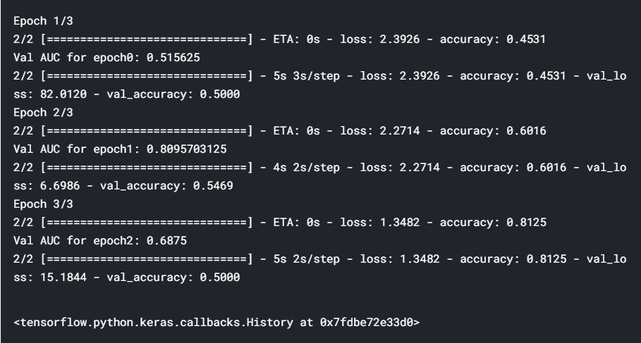

plt.imshow(image)

#standardizing image
#moved the origin to the centre of the image
h, w, _ = image.shape
img = image[int(h/2)-50:int(h/2)+50, int(w/2)-50:int(w/2)+50, : ]
model.predict(img[np.newaxis,: ])

Hey, we have got a very high probability for class 1 i.e. rose. If you remember, class 0 was daisy and class 1 was rose(on top of the blog). So, the model has learnt perfectly. We have built a model with a good AUC at the end of 3 epochs. If you train this using more epochs, you should be able to reach a better AUC value.

嘿，我們有很高的可能性上1類，即上升。 如果您還記得的話，班級0是雛菊，班級1是玫瑰(在博客頂部)。 因此，該模型學得很完美。 我們已經建立了一個模型，該模型在3個階段結束時具有良好的AUC。 如果您使用更多的時間進行訓練，則應該能夠達到更好的AUC值。

If you have any questions, recommendations or critiques, I can be reached via LinkedIn or the comment section.

如果您有任何疑問，建議或批評，請通過LinkedIn或評論欄與我聯系。