內部AI (Inside AI)

If you’ve steered clear of Bayesian regression because of its complexity, this article shows how to apply simple MCMC Bayesian Inference to linear data with outliers in Python, using linear regression and Gaussian random walk priors, testing assumptions on observation errors from Normal vs Student-T prior distributions and comparing against ordinary least squares.

如果您由于復雜性而避開了貝葉斯回歸，那么本文將介紹如何使用線性回歸和高斯隨機游走先驗，將簡單的MCMC貝葉斯推斷應用于帶有異常值的Python線性數據，測試來自Normal或Student的觀察誤差假設-T先驗分布，并與普通最小二乘法進行比較。

Ref: Jupyter Notebook and GitHub Repository

參考： Jupyter Notebook 和 GitHub存儲庫

The beauty of Bayesian methods is their ability to generate probability estimates of the quality of derived models based on a priori expectations of the behaviour of the model parameters. Rather than a single point-solution, we obtain a distribution of solutions each with an assigned probability. A priori expectations of the data behaviour are formulated into a set of Priors, probability distributions over the model parameters.

的T貝葉斯方法，他的美是他們產生衍生車型的基礎上，模型參數的行為的先驗預期質量的概率估計能力。 而不是單點解，我們獲得了具有指定概率的解的分布。 數據行為的先驗期望被公式化為一組Priors ，即模型參數上的概率分布。

The following scenario is based on Thomas Wiecki’s excellent article “GLM: Robust Linear Regression”1 and is an exploration of the Python library PyMC32 as a means to model data using Markov chain Monte Carlo (MCMC) methods in Python, with some discussion of the predictive power of the derived Bayesian models. Different priors are considered, including Normal, Student-T, Gamma and Gaussian Random Walk, with a view to model the sample data both using generalized linear models (GLM) and by taking a non-parametric approach, estimating observed data directly from the imputed priors.

以下場景基于Thomas Wiecki的出色文章“ GLM：穩健的線性回歸”1，并且是對Python庫PyMC32的探索，該方法是使用Python中的馬爾可夫鏈蒙特卡洛(MCMC)方法對數據進行建模的一種方法，并進行了一些討論。貝葉斯模型的預測能力。 考慮了不同的先驗，包括法線，Student-T，伽馬和高斯隨機游走，以期使用廣義線性模型(GLM)并通過采用非參數方法對樣本數據建模，從而直接從推算中估算觀察到的數據先驗。

樣本數據 (Sample Data)

Our sample data is generated as a simple linear model with given intercept and slope, with an additional random Gaussian noise term added to each observation. To make the task interesting, a small number of outliers are added to the distribution which have no algebraic relationship to the true linear model. Our objective is to model the observed linear model as closely as possible with the greatest possible robustness to disruption by the outliers and the observation error terms.

我們的樣本數據是作為具有給定截距和斜率的簡單線性模型生成的，每個觀察值都添加了一個額外的隨機高斯噪聲項。 為了使任務有趣，向分布中添加了少量離群值，這些離群值與真實線性模型沒有代數關系。 我們的目標是盡可能密切地建模觀察到的線性模型，以最大程度地增強對異常值和觀察誤差項的干擾。

普通與學生T先驗 (Normal vs Student-T priors)

We compare models based on Normal versus Student-T observation error priors. Wiecki shows that a Student-T prior is better at handling outliers than the Normal as the distribution has longer tails, conveying the notion that an outlier is not to be considered wholly unexpected.

我們比較基于正常與學生-T觀察誤差先驗的模型。 Wiecki表示，由于分布的尾部較長，因此Student-T先驗值在處理異常值方面要比正態值更好，這表達了一個觀點，即異常值不應被視為完全出乎意料。

真線性模型和普通最小二乘(OLS)回歸 (True linear model and Ordinary Least Squares (OLS) regression)

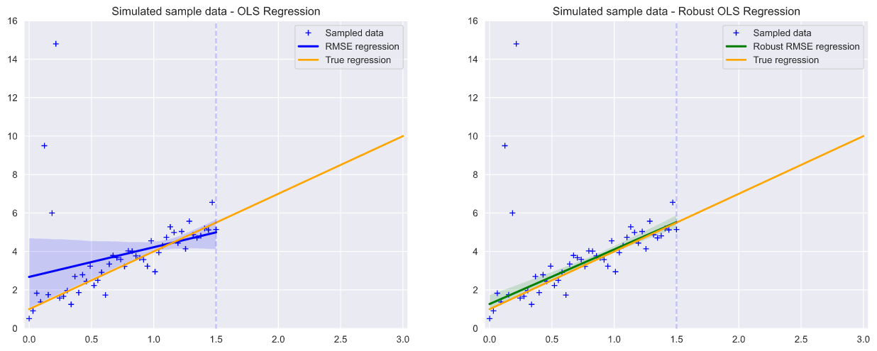
def add_outliers(y, outliers_x, outliers_y):y_observed = yfor i in range(len(outliers_x)):y_observed[outliers_x[i]] = outliers_y[i]y_predicted = np.append(y_observed, [0] * observables)y_predicted = np.ma.MaskedArray(y_predicted,np.arange(y_predicted.size)>=observables)return y_observed, y_predictedx_observed = np.linspace(0, 1.5, observables)
x_delta = np.linspace(1.5, 3.0, observables)
x_predicted = np.append(x_observed, x_delta)predicted_line = true_intercept + true_slope * x_predictedy = true_intercept + true_slope * x_observed + np.random.default_rng(seed=123).normal(scale=0.5, size=observables) # Add noisey_observed, y_predicted = add_outliers(y, outliers_x, outliers_y)

def plot_sample_data(ax, y_min, y_max):ax.set_xlim(-0.04, 3.04)ax.set_ylim(y_min, y_max)plt.plot(x_predicted, y_predicted, '+', label='Sampled data', c=pal_2[5])def plot_true_regression_line(title, loc):plt.plot(x_predicted, predicted_line, lw=2., label = 'True regression', c='orange')plt.axvline(x=x_predicted[observables],linestyle='--', c='b',alpha=0.25)plt.title(title)plt.legend(loc=loc)data = dict(x=x_observed, y=y_observed)
fig = plt.figure(figsize=(fig_size_x, fig_size_y))
ax1 = fig.add_subplot(121)
plot_sample_data(ax1, y_min_compact, y_max_compact)
seaborn.regplot(x="x", y="y", data=data, marker="+", color="b", scatter=False, label="RMSE regression")
plot_true_regression_line('Simulated sample data - OLS Regression', 'best')ax2 = fig.add_subplot(122)
plot_sample_data(ax2, y_min_compact, y_max_compact)
seaborn.regplot(x="x", y="y", data=data, marker="+", color="g", robust=True, scatter=False, label="Robust RMSE regression")
plot_true_regression_line('Simulated sample data - Robust OLS Regression', 'best')

We start with a simulated dataset of observations of the form y=ax+b+epsilon, with the noise term epsilon drawn from a normal distribution. Here we 1) create observation values in the range x from 0 to 1.5, based on the ‘true’ linear model, 2) add test outliers and 3) extend the x axis from 1.5 to 3.0 so we can test the predictive power of our models into this region.

我們從y = ax + b + epsilon形式的觀測數據的模擬數據集開始，噪聲項epsilon從正態分布中得出。 在這里，我們1)基于“真實”線性模型創建介于0到1.5范圍內的x的觀測值，2)添加測試異常值，3)將x軸從1.5擴展到3.0以測試我們的預測能力建模到該區域。

In the predictive region we have used numpy.MaskedArray() function in order to indicate to PyMC3 that we have unknown observational data in this region1?.

在預測區域中，我們使用了numpy.MaskedArray()函數來向PyMC3指示在該區域中我們未知的觀測數據。

It is useful to visualize the simulated data, along with the true regression line and ordinary least squares regression.

可視化模擬數據以及真實的回歸線和普通的最小二乘回歸非常有用。

The Seaborn library allows us to draw this plot directly?, and we can also set a ‘robust’ flag which calculates the regression line while de-weighting outliers.

Seaborn庫允許我們直接繪制此圖?，我們還可以設置一個“ robust ”標志，該標志在對異常值進行加權時計算回歸線。

PyMC3的貝葉斯回歸 (Bayesian Regression with PyMC3)

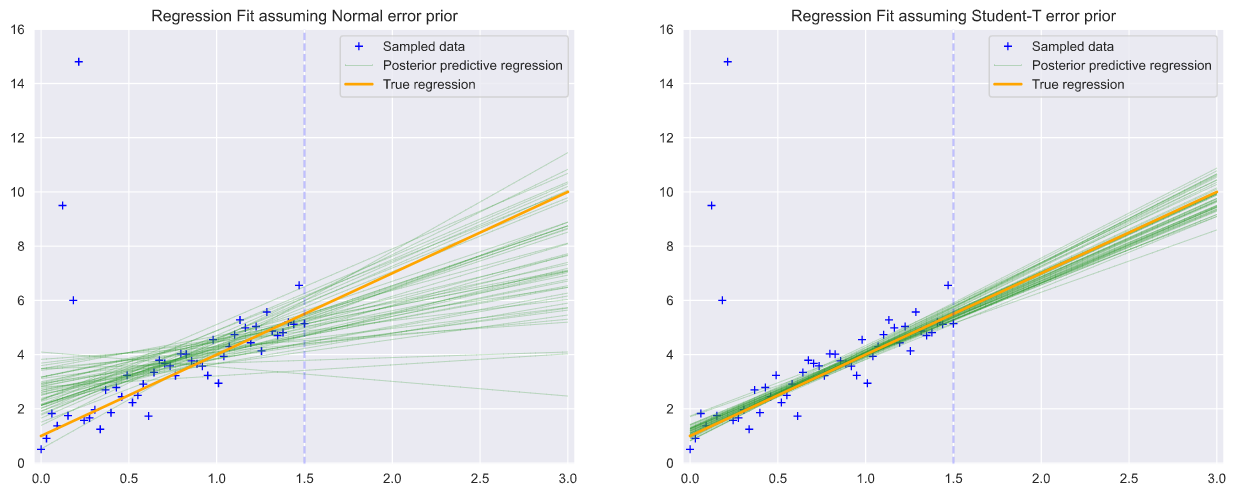
Following the example of Wiecki, we can create linear regression models (GLM) in PyMC3, generating the linear model from y(x)= ‘y ~ x’.

?Following Wiecki的例子中，我們可以創建線性回歸模型(GLM)在PyMC3，生成從y中(x)的線性模型= 'Y?X'。

To test the notion of robust regression, we create two models, one based on a Normal prior of observational errors and a second based on the Student-T distribution, which we expect to be less influenced by outliers.

為了測試魯棒回歸的概念，我們創建了兩個模型，一個模型基于觀測誤差的正態先驗，另一個模型基于Student-T分布，我們希望它們不受異常值的影響較小。

data = dict(x=x_observed, y=y_observed)
with pm.Model() as n_model:pm.glm.GLM.from_formula('y ~ x', data)trace_normal_glm = pm.sample(samples_glm, tune=tune_glm, random_seed=123, cores=2, chains=2)with pm.Model() as t_model:pm.glm.GLM.from_formula('y ~ x', data, family = pm.glm.families.StudentT())trace_studentT_glm = pm.sample(samples_glm, tune=tune_glm, random_seed=123, cores=2, chains=2)

fig = plt.figure(figsize=(fig_size_x, fig_size_y))
ax1 = fig.add_subplot(121)
plot_sample_data(ax1, y_min_compact, y_max_compact)
pm.plot_posterior_predictive_glm(trace_normal_glm, eval=x_predicted, samples=50, label='Posterior predictive regression', c=pal_1[4])
plot_true_regression_line('Regression Fit assuming Normal error prior', 'best')ax2 = fig.add_subplot(122)
plot_sample_data(ax2, y_min_compact, y_max_compact)
pm.plot_posterior_predictive_glm(trace_studentT_glm, eval=x_predicted, samples=50, label='Posterior predictive regression', c=pal_1[4])
plot_true_regression_line('Regression Fit assuming Student-T error prior', 'best')

The pymc3.sample() method allows us to sample conditioned priors. In the case of the Normal model, the default priors will be for intercept, slope and standard deviation in epsilon. In the case of the Student-T model priors will be for intercept, slope and lam?.

pymc3.sample()方法允許我們采樣條件先驗。 在普通模型的情況下，默認優先級將用于ε，ε的截距，斜率和標準偏差。 對于Student-T模型，先驗將用于截距，斜率和lam。

Running these two models creates trace objects containing a family of posteriors sampled for each model over all chains, conditioned on the observations, from which we we can plot individual glm regression lines.

運行這兩個模型將創建一個跟蹤對象，該跟蹤對象包含所有鏈上每個模型采樣的后驗對象，并以觀測為條件，從中我們可以繪制單個glm回歸線。

正態誤差與Student-T誤差分布的比較 (Comparison of Normal vs Student-T error distributions)

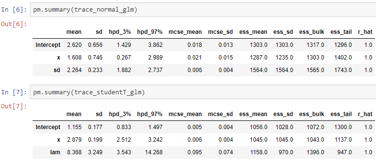
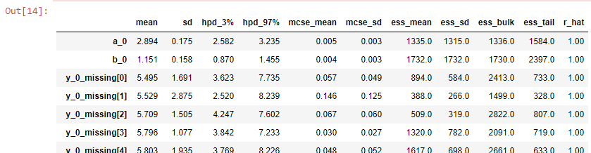
A summary of the parameter distributions can be obtained from pymc3.summary(trace) and we see here that the intercept from the Student-T prior is 1.155 with slope 2.879. Hence much closer to the expected values of 1, 3 than those from the Normal prior, which gives intercept 2.620 with slope 1.608.

可以從pymc3.summary(trace)獲得參數分布的摘要，我們在這里看到來自Student-T先驗的截距為1.155 ，斜率為2.879。 因此，與正常先驗的期望值相比，更接近于1、3的期望值，即截距2.620的斜率為1.608 。

完善Student-T錯誤分布 (Refinement of Student-T error distribution)

It is clear from the plots above that we have improved the regression by using a Student-T prior, but we we hope to do better by refining the Student-T degrees of freedom parameter.

這是從上面我們已經改善了現有使用Student-T的回歸情節清楚，但我們希望大家通過細化學生-T自由度參數做的更好。

def create_normal_glm_model(samples, tune, x, y):with pm.Model() as model_normal:a_0 = pm.Normal('a_0', mu=1, sigma=10)b_0 = pm.Normal('b_0', mu=1, sigma=10)mu_0 = a_0 * x + b_0sigma_0 = pm.HalfCauchy('sigma_0', beta=10)y_0 = pm.Normal('y_0', mu=mu_0, sigma=sigma_0, observed=y)trace_normal = pm.sample(samples, tune=tune, random_seed=123, cores=2, chains=2)return trace_normal, pm.sample_posterior_predictive(trace_normal, random_seed=123)['y_0']def create_studentT_glm_model(samples, tune, x, y):with pm.Model() as model_studentT:a_0 = pm.Normal('a_0', mu=1, sigma=10)b_0 = pm.Normal('b_0', mu=1, sigma=10)mu_0 = a_0 * x + b_0nu_0 = pm.Gamma('nu_0', alpha=2, beta=0.1)y_0 = pm.StudentT('y_0', mu=mu_0, lam=8.368, nu=nu_0, observed=y)trace_studentT = pm.sample(samples, tune=tune, random_seed=123, cores=2, chains=2)return trace_studentT, pm.sample_posterior_predictive(trace_studentT, random_seed=123)['y_0']trace_normal_glm_explicit, y_posterior_normal_glm = create_normal_glm_model(samples_glm, tune_glm, x_observed, y_observed)
trace_studentT_glm_explicit, y_posterior_studentT_glm = create_studentT_glm_model(samples_glm, tune_glm, x_observed, y_observed)

Models: The distribution for the Normal model’s standard deviation prior is a HalfCauchy, a positive domain Student-T with one degree of freedom1?, which mirrors our previous model.

模型：常規模型的標準偏差之前的分布是HalfCauchy，這是一個具有一個自由度的正Student-T域，與我們的先前模型類似。

We also need to construct a new Student-T model where as well as parameterizing the glm we also create a prior on nu, the degrees of freedom parameter.

我們還需要構造一個新的Student-T模型，在參數化glm的同時，還要在nu (自由度參數)上創建先驗。

nu is modelled as a Gamma function, as recommended by Andrew Gelman? nu ~ gamma(alpha=2, beta=0.1), and retaining the lam value of 8.368 from the run above.

nu被建模為Gamma函數，正如AndrewGelman?nu?gamma(alpha = 2，beta = 0.1)所建議的那樣，并且從上述運行中保留了lam值為8.368。

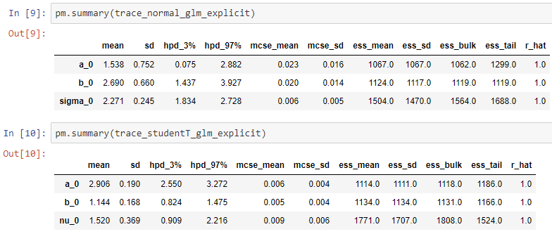
Results: From summary(trace) we can see that the intercept from the Student-T error distribution is improved to 1.144, with slope 2.906 against the previous result of 1.155, with slope 2.879.

結果：從摘要(痕量)，我們可以看到，從學生-T誤差分布截距提高到1.144，用斜率2.906針對1.155先前的結果，具有斜率2.879。

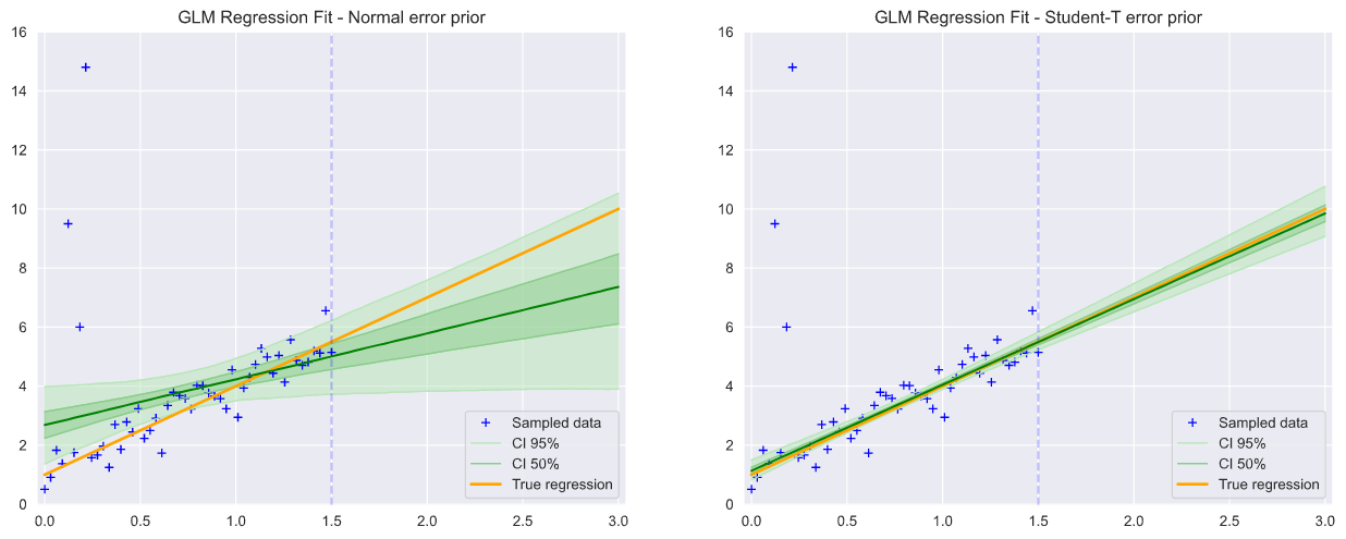
def calculate_regression_line(trace):a0 = trace['a_0']b0 = trace['b_0']y_pred = np.array([])for x_i in x_predicted:y_quartiles = np.percentile(a0 * x_i + b0, quartiles)y_pred = np.append(y_pred, y_quartiles)return np.transpose(y_pred.reshape(len(x_predicted), no_quartiles))

def plot_intervals(ax, y_pred, title, pal, loc, y_min, y_max):plt.fill_between(x_predicted,y_pred[0,:],y_pred[4,:],alpha=0.5, color=pal[1])plt.fill_between(x_predicted,y_pred[1,:],y_pred[3,:],alpha=0.5, color=pal[2])plot_intervals_line(ax, y_pred, title, pal, loc, 1, y_min, y_max)def plot_intervals_line(ax, y_pred, title, pal, loc, lw, y_min, y_max):plot_sample_data(ax, y_min, y_max)plt.plot(x_predicted, y_pred[0,:], label='CI 95%', lw=lw, c=pal[1])plt.plot(x_predicted, y_pred[4,:], lw=lw, c=pal[1])plt.plot(x_predicted, y_pred[1,:], label='CI 50%', lw=lw, c=pal[2])plt.plot(x_predicted, y_pred[3,:], lw=lw, c=pal[2])plot_true_regression_line(title, loc)def plot_regression(y_pred_normal, y_pred_student, loc, y_min, y_max):fig = plt.figure(figsize=(fig_size_x, fig_size_y))ax1 = fig.add_subplot(121)plot_intervals(ax1, y_pred_normal, 'GLM Regression Fit - Normal error prior', pal_1, loc, y_min, y_max)plt.plot(x_predicted, y_pred_normal[2,:], c=pal_1[5],label='Posterior regression')ax2 = fig.add_subplot(122)plot_intervals(ax2, y_pred_student, 'GLM Regression Fit - Student-T error prior', pal_1, loc, y_min, y_max)plt.plot(x_predicted, y_pred_student[2,:], c=pal_1[5], label='Posterior regression')y_pred_normal_glm = calculate_regression_line(trace_normal_glm_explicit)
y_pred_studentT_glm = calculate_regression_line(trace_studentT_glm_explicit)plot_regression(y_pred_normal_glm, y_pred_studentT_glm, 4, y_min_compact, y_max_compact)

Visualizing credibility intervals: Having fitted the linear models and obtained intercept and slope for every sample we can calculate expected y(x) at every point on the x axis and then use numpy.percentile() to aggregate these samples into credibility intervals (CI)? on x.

可視化可信區間：擬合線性模型并獲得每個樣本的截距和斜率，我們可以計算x軸上每個點的預期y(x) ，然后使用numpy.percentile()將這些樣本匯總為可信區間(CI) ?在x上 。

We can visualize the mean, 50% and 95% credibility intervals of the sampled conditioned priors as all values for all Markov chains are held in the trace object. It is clear below how close the credibility intervals lie to the true regression for the Student-T model.

由于所有馬爾可夫鏈的所有值都保存在跟蹤對象中，因此我們可以可視化采樣條件條件先驗的均值，50％和95％可信區間。 從下面可以清楚地看出，可信區間與Student-T模型的真實回歸有多接近。

Later in this article we consider a non-parametric model which follows the linear trend line while modelling fluctuations in observations, which can convey local information which we might wish to preserve.

在本文的稍后部分，我們將考慮一個遵循線性趨勢線的非參數模型，同時對觀測值的波動建模，可以傳達我們可能希望保留的局部信息。

后驗預測力 (Posterior predictive power)

Bayesian inference works by seeking modifications to the parameterized prior probability distributions in order to maximise a likelihood function of the observed data over the prior parameters.

乙 ayesian推理作品通過尋求為了最大化比現有參數觀測數據的似然函數的修改的參數先驗概率分布。

So what happens to the expected posterior in regions where we have missing sample data? We should find that the posterior predictions follow the regression line, taking into account fluctuations due to the error term.

那么，在缺少樣本數據的區域中，預期后驗會如何處理？ 考慮到誤差項引起的波動，我們應該發現后驗預測遵循回歸??線。

建模未觀察到的數據 (Modelling unobserved data)

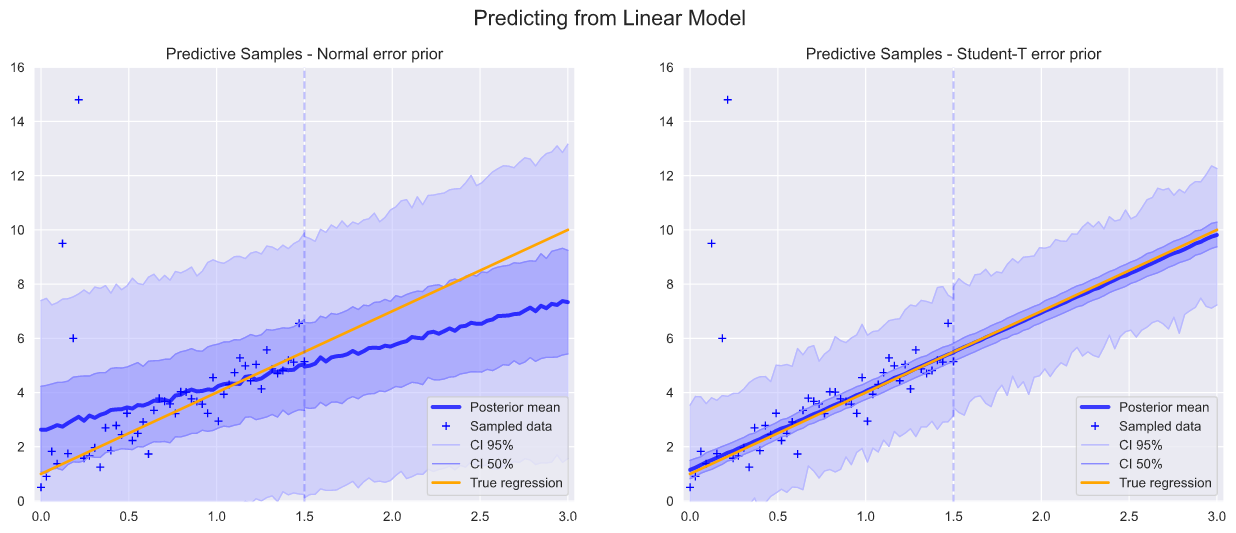
We have created a y_predicted array of observations which in the region 1.5 to 3 is masked, indicating that these are unobserved samples. PyMC3 adds these missing observations as new priors, y_missing, and computes a posterior distribution over the full sample space.

我們創建了一個y_predicted觀測值數組，該數組在1.5到3的范圍內被遮罩，表明這些是未觀察到的樣本。 PyMC3將這些缺失的觀測值添加為新的先驗y_missing ，并計算整個樣本空間的后驗分布。

trace_normal_glm_pred, y_posterior_normal_glm_pred = create_normal_glm_model(samples_glm, tune_glm, x_predicted, y_predicted)
trace_studentT_glm_pred, y_posterior_studentT_glm_pred = create_studentT_glm_model(samples_glm, tune_glm, x_predicted, y_predicted)pm.summary(trace_studentT_glm_pred)

Re-running the above models with this extended sample space yields statistics which now include the imputed, observations.

在擴展的樣本空間下重新運行上述模型將產生統計信息，其中包括估算的觀測值。

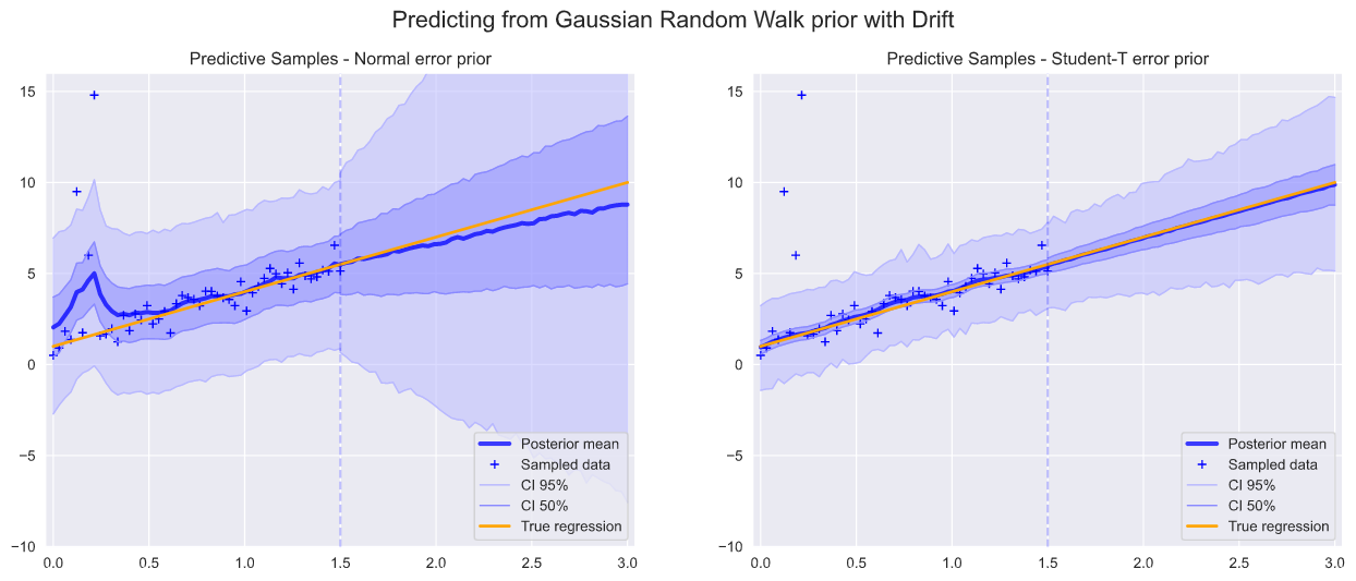
def plot_actuals(y_posterior_normal, y_posterior_student, loc, y_min, y_max):y_pred_normal = np.percentile(y_posterior_normal, quartiles, axis=0)y_pred_studentT = np.percentile(y_posterior_student, quartiles, axis=0)fig = plt.figure(figsize=(fig_size_x, fig_size_y))ax1 = fig.add_subplot(121)plt.plot(x_predicted, y_pred_normal[2,:],alpha=0.75, lw=3, color=pal_2[5],label='Posterior mean')plot_intervals(ax1, y_pred_normal, 'Predictive Samples - Normal error prior', pal_2, loc, y_min, y_max)ax2 = fig.add_subplot(122)plt.plot(x_predicted, y_pred_studentT[2,:],alpha=0.75, lw=3, color=pal_2[5],label='Posterior mean')plot_intervals(ax2, y_pred_studentT, 'Predictive Samples - Student-T error prior', pal_2, loc, y_min, y_max)return figfig = plot_actuals(y_posterior_normal_glm_pred, y_posterior_studentT_glm_pred, 4, y_min_compact, y_max_compact)
fig.suptitle('Predicting from Linear Model', fontsize=16)

When we run this model we see in the summary not only the priors for a0, b0, nu0 but also for all the missing y, as y_0_missing.

當我們運行該模型時，我們在摘要中不僅看到a0，b0，nu0的先驗，而且還看到所有缺失的y，如y_0_missing。

Having inferred the full range of predicted sample observations we can plot these posterior means, along with credibility intervals.

推斷出預測樣本觀察的全部范圍后，我們可以繪制這些后驗均值以及可信區間。

We see below that the inferred observations have been well fitted to the expected linear model.

我們在下面看到，推斷的觀測值已經很好地擬合了預期的線性模型。

非參數推理模型 (Non-parametric Inference Models)

Having verified the linear model, it would be nice to see if we can model these sample observations with a non-parametric model, where we dispense with finding intercept and slope parameters and instead try to model the observed data directly with priors on every datapoint across the sample space11.

?AVING驗證線性模型，這將是很好看，如果我們可以用一個非參數模型，其中我們用查找截距和斜率參數分配這些樣本觀測模型，而是嘗試將觀察到的數據直接與每一個數據點先驗模型整個樣品空間11。

非平穩數據和先驗隨機走動12 (Non-Stationary data and Random Walk prior12)

The simple assumption with a non-parametric model is that the data is stationary, so the observed samples at each datapoint do not trend in a systematic way.

使用非參數模型的簡單假設是數據是固定的，因此在每個數據點觀察到的樣本不會以系統的方式趨向。

def create_normal_stationary_inference_model(samples, tune, y):with pm.Model() as model_normal:sigma_0 = pm.HalfCauchy('sigma_0', beta=10)sigma_1 = pm.HalfCauchy('sigma_1', beta=10)mu_0 = pm.Normal('mu_0', mu=0, sd=sigma_1, shape=y.size)y_0 = pm.Normal('y_0', mu=mu_0, sd=sigma_0, observed=y)trace = pm.sample(samples, tune=tune, random_seed=123, cores=2, chains=2)return trace, pm.sample_posterior_predictive(trace, random_seed=123)['y_0']def create_studentT_stationary_inference_model(samples, tune, y):with pm.Model() as model_studentT:nu_0 = pm.Gamma('nu_0', alpha=2, beta=0.1)sigma_1 = pm.HalfCauchy('sigma_1', beta=10)mu_0 = pm.Normal('mu_0', mu=0, sd=sigma_1, shape=y.size)y_0 = pm.StudentT('y_0', mu=mu_0, lam=8.368, nu=nu_0, observed=y)trace =  pm.sample(samples, tune=tune, random_seed=123, cores=2, chains=2)return trace, pm.sample_posterior_predictive(trace, random_seed=123)['y_0']

But real-world data does very often trend, or is at least constrained by requirements of smoothness to adjacent data points and then the choice of priors is crucial13.

但是，現實世界中的數據確實經常會趨勢化，或者至少受到對相鄰數據點的平滑度要求的限制，然后選擇先驗至關重要。

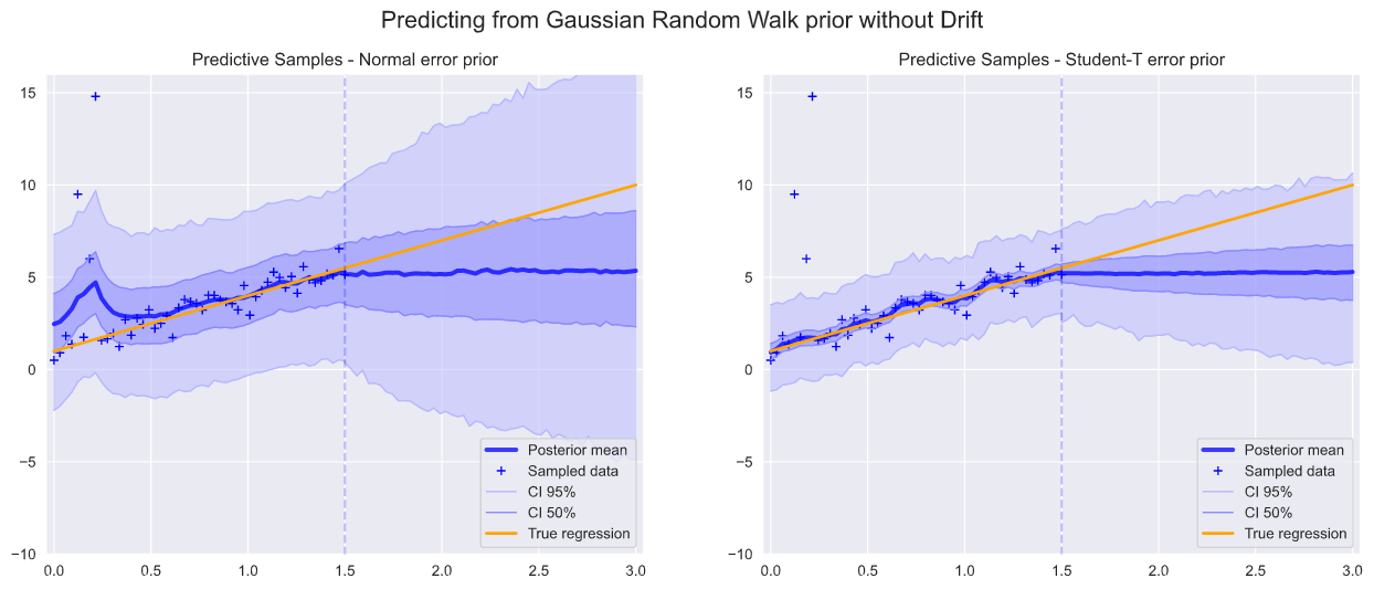
In our scenario the data is non-stationary, since it has a clear trend over x. If we use a simple gaussian prior for our observations, then even after conditioning with the observed data, as soon as we enter the unobserved region, the predicted observations rapidly return to their prior mean.

在我們的場景中，數據是不穩定的，因為在x上有明顯的趨勢。 如果我們使用簡單的高斯先驗進行觀察，那么即使在對觀察到的數據進行條件調整之后，只要我們進入未觀察到的區域，預測的觀察就會Swift返回到其先前的均值。

高斯隨機游走先驗 (Gaussian Random Walk prior)

Gaussian random walk prior gives us the ability to model non-stationary data because it estimates an observable based on the previous data point state plus a random walk step. The PyMC3 implementation also allows us to model a drift parameter which adds a fixed scalar to each random walk step.

摹 aussian隨機游走之前讓我們來模擬非平穩數據的能力，因為它的估計基于先前的數據點的狀態加上一個隨機游走一步可觀察到的。 PyMC3的實現還允許我們對漂移參數建模，該參數為每個隨機步階添加了一個固定的標量。

def create_normal_grw_inference_model(samples, tune, y, drift):with pm.Model() as model_normal:sigma_0 = pm.HalfCauchy('sigma_0', beta=10)sigma_1 = pm.HalfCauchy('sigma_1', beta=10)if drift:mu_drift = pm.Normal('mu_drift', mu=1, sigma=2)mu_0 = pm.GaussianRandomWalk('mu_0', mu=mu_drift, sd=sigma_1, shape=y.size)else:mu_0 = pm.GaussianRandomWalk('mu_0', mu=0, sd=sigma_1, shape=y.size)y_0 = pm.Normal('y_0', mu=mu_0, sd=sigma_0, observed=y)trace = pm.sample(samples, tune=tune, random_seed=123, cores=2, chains=2)return trace, pm.sample_posterior_predictive(trace, random_seed=123)['y_0']def create_studentT_grw_inference_model(samples, tune, y, drift):with pm.Model() as model_studentT:nu_0 = pm.Gamma('nu_0', alpha=2, beta=0.1)sigma_1 = pm.HalfCauchy('sigma_1', beta=10)if drift:mu_drift = pm.Normal('mu_drift', mu=1, sigma=2)mu_0 = pm.GaussianRandomWalk('mu_0', mu=mu_drift, sd=sigma_1, shape=y.size)else:mu_0 = pm.GaussianRandomWalk('mu_0', mu=0, sd=sigma_1, shape=y.size)y_0 = pm.StudentT('y_0', mu=mu_0, lam=8.368, nu=nu_0, observed=y)trace =  pm.sample(samples, tune=tune, random_seed=123, cores=2, chains=2)return trace, pm.sample_posterior_predictive(trace, random_seed=123)['y_0']

In these two inference models we have used a single scalar drift parameter which in this scenario is equivalent to the slope on the data in the direction of the drift.

在這兩個推理模型中，我們使用了單個標量漂移參數，在這種情況下，該參數等于數據在漂移方向上的斜率。

It is important that data, including outliers, is correctly ordered with equal sample step size, as the prior will assume this behaviour in modelling the data. For this reason outliers are inserted into x array at index points, not appended as (x, y).

重要的是，必須以相等的樣本步長大小正確排序數據(包括異常值)，因為先驗者將在建模數據時采用這種行為。 因此，離群值在索引點處插入 x數組中， 而不附加為(x，y)。

Below we run the two models, first with the drift parameter set to zero, leading to a static line at the last observation point, and second with the drift inferred from the data.

下面我們運行兩個模型，第一個模型的漂移參數設置為零，在最后一個觀察點指向一條靜態線，第二個模型從數據推斷出的漂移。

As can be seen, this final model gives a very nice fit to the linear trend, particularly when using the Student-T prior which is less influenced by the outliers.

可以看出，該最終模型非常適合線性趨勢，尤其是在使用Student-T優先級時，該值不受異常值的影響較小。

繪制高斯隨機游走的后驗樣本 (Plot posterior samples from Gaussian random walk)

def plot_samples(y_posterior, samples):show_label = Truefor rand_loc in np.random.randint(0, len(y_posterior), samples):rand_sample = y_posterior[rand_loc]if show_label:plt.plot(x_predicted, rand_sample, alpha=0.05, c=pal_1[5], label='Posterior samples')show_label = Falseelse:plt.plot(x_predicted, rand_sample, alpha=0.05, c=pal_1[5])def plot_posterior_predictive(y_posterior_normal, y_posterior_student, loc, samples, y_min, y_max):y_pred_normal = np.percentile(y_posterior_normal, quartiles, axis=0)y_pred_studentT = np.percentile(y_posterior_student, quartiles, axis=0)fig = plt.figure(figsize=(fig_size_x, fig_size_y))ax1 = fig.add_subplot(121)plot_samples(y_posterior_normal, samples)plt.plot(x_predicted, y_pred_normal[2,:], alpha=0.75, lw=3, color=pal_2[5], label='Posterior mean')plot_intervals_line(ax1, y_pred_normal, 'Random Walk Prior: Predictive Samples - Normal error prior', pal_2, loc, 2, y_min, y_max)ax2 = fig.add_subplot(122)plot_samples(y_posterior_student, samples)plt.plot(x_predicted, y_pred_studentT[2,:], alpha=0.75, lw=3, color=pal_2[5], label='Posterior mean')plot_intervals_line(ax2, y_pred_studentT, 'Random Walk Prior: Predictive Samples - Student-T error prior', pal_2, loc, 2, y_min, y_max)plot_posterior_predictive(y_posterior_normal, y_posterior_studentT, 4, 250, y_min_spread, y_max_compact)pm.traceplot(trace_studentT)

Also, we now have the benefit that we can see the effect of the outliers in local perturbations to linearity.

而且，我們現在有一個好處，就是可以看到離群值在局部擾動對線性的影響。

Below we visualize some of the actual random walk samples.

下面我們可視化一些實際的隨機游動樣本。

We should not expect any particular path to be close to the actual predicted path of our sample data. In this sense it is a truly stochastic method as our result is derived from the statistical mean of the sampled paths, not from any particular sample’s path.

我們不應期望任何特定路徑接近我們樣本數據的實際預測路徑。 從這個意義上說，這是一種真正的隨機方法，因為我們的結果是從采樣路徑的統計平均值中得出的，而不是從任何特定樣本的路徑中得出的。

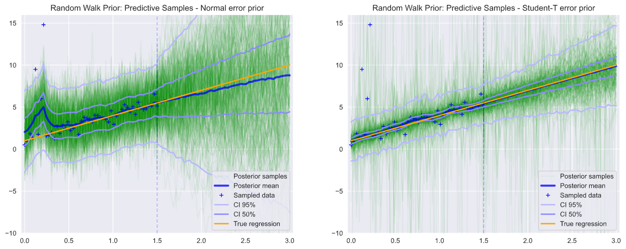
離群值對隨機游走預測后驗的影響 (Impact of Outliers on Random Walk predictive posteriors)

# Remove the outliers
y = true_intercept + true_slope * x_observed + np.random.default_rng(seed=123).normal(scale=0.5, size=observables) # Add noisey_observed, y_predicted = add_outliers(y, [], [])trace_normal, y_posterior_normal_linear = create_normal_grw_inference_model(samples_predictive, tune_predictive, y_predicted, True) # With Drift
trace_studentT, y_posterior_studentT_linear = create_studentT_grw_inference_model(samples_predictive, tune_predictive, y_predicted, True) # With Drift

Having seen the effect that the outliers have on the posterior mean, we surmise that the noisiness of the predictive samples might be due to perturbation of the random walk caused by the outliers.

看到離群值對后均值的影響后，我們推測預測樣本的噪聲可能是由于離群值引起的隨機游走擾動。

To test this, we have here removed the outliers and rerun the same two predictive models.

為了測試這一點，我們在這里刪除了異常值，然后重新運行相同的兩個預測模型。

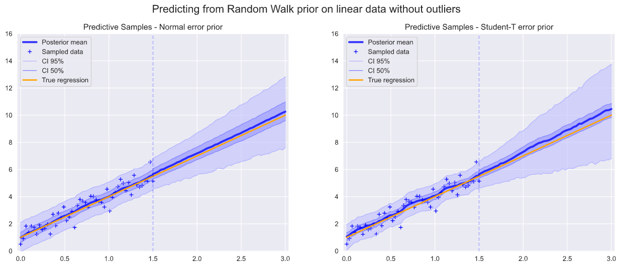
As can be seen, the predictive samples are much cleaner, with very tight credibility intervals and much smaller divergence in the random walk samples. This gives us confidence that with a correct model the Gaussian random walk is a well conditioned prior for non-stationary model fitting.

可以看出，預測樣本更干凈，可信區間非常緊密，隨機游走樣本的差異小得多。 這使我們相信，使用正確的模型，高斯隨機游走是非平穩模型擬合之前的良好條件。

結論 (Conclusion)

The intention of this article was to show the simplicity and power of Bayesian learning with PyMC3 and hopefully we have:

本文的目的是展示使用PyMC3進行貝葉斯學習的簡單性和功能，希望我們有：

• shown that the Student-T error prior performs better that the Normal prior in robust linear regression;
  表明在穩健線性回歸中，Student-T誤差先驗比正常先驗表現更好；
• demonstrated that the refined degrees of freedom on the Student-T error prior improves the fit to the regression line;
  證明了對Student-T錯誤的改進后的自由度提高了對回歸線的擬合度；
• shown we can quickly and easily draw credibility intervals on the posterior samples for both the linear regression and the non-parametric models;
  表明我們可以在線性樣本和非參數模型上快速輕松地在后驗樣本上繪制可信區間；
• demonstrated that the non-parametric model using Gaussian random walk with drift can predict the linear model in unobserved regions and at the same time allow model local fluctuations in the observed data which we might want to preserve;
  證明了使用帶有漂移的高斯隨機游走的非參數模型可以預測未觀測區域的線性模型，同時允許我們可能希望保留的觀測數據中的模型局部波動；
• investigated the Gaussian random walk prior and shown that its chaotic behaviour allows it to explore a wide sample space while not preventing it generating smooth predictive posterior means.
  對高斯隨機游走進行了先驗研究，結果表明其混沌行為使其能夠探索廣闊的樣本空間，同時又不會阻止其生成平滑的預測后驗均值。

Thanks for reading, please feel free to add comments or corrections. Full source code can be found in the Jupyter Notebook and GitHub Repository.

感謝您的閱讀，請隨時添加評論或更正。 完整的源代碼可以在Jupyter Notebook和GitHub Repository中找到 。