97%. That’s the percentage of data that sits unused by organizations according to Gartner, making up so-called “dark data”.

97 ％。 根據Gartner的說法，這就是組織未使用的數據百分比，即所謂的“ 暗數據 ”。

Data has overtaken oil as the world’s most valuable resource, but nearly all of it is still unused by organizations. Gartner estimates that 87% of organizations have “low BI and analytics maturity”.

數據已取代石油成為世界上最有價值的資源，但幾乎所有組織仍未使用它。 Gartner估計，87％的組織具有“較低的BI和分析成熟度”。

A possible explanation for this paradox is that not all data are created equal. The value of data can vary drastically from one organization to another, and within the same organization from one project to another.

對于這種悖論的一種可能解釋是，并非所有數據都是相同的。 數據的價值在一個組織與另一個組織之間可能會發生巨大變化，而在同一組織內，一個項目與另一個項目之間的數據價值可能會發生巨大變化。

In order to make the required investment in business intelligence and analytics, organizations should be able to anticipate, to an accurate degree, the business impact of doing so, and such a future investment should be expected to yield a high enough ROI.

為了在商業智能和分析上進行所需的投資，組織應該能夠準確地預測這樣做的業務影響，并且這種未來的投資應該產生足夠高的ROI。

Data Cannot Become the New Oil Without The Machine Learning Equivalent of Exploration Geophysics

沒有探索地球物理的機器學習等效性，數據就無法成為新石油

Assuming that data is always valuable and attempting to extract such value by trial-and-error as part of an AI project, be it driven by an AutoML platform, can be very wasteful at best, and have a negative ROI in the worst-case scenario.

假設數據始終是有價值的，并嘗試通過試錯法將其作為AI項目的一部分來提取，這是由AutoML平臺驅動的，充其量是非常浪費的，在最壞的情況下，其ROI為負場景。

Pursuant to the oil analogy, this would be equivalent to assuming that there is always oil in the ground wherever one looks and that the only factor driving the amount of oil extracted from the ground is the extraction technique one uses.

根據該油的比喻，這將等同于假定總是有油在地面的地方一個外觀和其驅動的油從地下提取的量的唯一因素是萃取技術一個用途。

Over the years, an entire field of study at the intersection of geophysics and economics, namely exploration geophysics, has been devoted to reducing the business risk in oil production. Exploration geophysics relies on inductive reasoning (as opposed to deductive reasoning) to detect the presence of and to estimate the amount of valuable geological deposits at a given location, without incurring the upfront cost and risk of building an exploitation site.

多年來，地球物理與經濟學交叉領域的整個研究領域，即勘探地球物理 ，一直致力于降低石油生產中的商業風險。 勘探地球物理學依靠歸納推理 (與演繹推理相對)來檢測給定位置的存在并估算有價值的地質礦床的數量，而不會產生前期成本和建設開發場地的風險。

Similarly, in order to reduce the business risk in investing in AI projects, it is crucial to develop inductive reasoning methods for quantifying the value of data, prior to and independently from doing any predictive modeling, a phase we refer to as pre-learning.

同樣，為了降低投資AI項目的業務風險，至關重要的是在進行任何預測建模之前并獨立于其進行預測，開發歸納推理方法來量化數據的價值，這一階段我們稱為預學習 。

Whereas the deductive approach for valuing a dataset would consist of first allocating resources to put the dataset to use and then monitoring the business impact for a while, the inductive approach consists of using mathematical reasoning to infer from the dataset of interest the highest performance that can be achieved by any predictive model, inexpensively, and without having to train any predictive model.

評估數據集的演繹方法包括首先分配資源以使用該數據集，然后監視一段時間的業務影響，而歸納法則包括使用數學推理從感興趣的數據集中推斷出可以實現的最高性能。可以通過任何預測模型廉價地實現，而無需訓練任何預測模型。

In this article, we summarize the theoretical foundations that enable pre-learning, and we illustrate how to quantify the juice in various datasets using the open-source kxy python package.

在本文中，我們總結了啟用預學習的理論基礎，并說明了如何使用開源kxy python軟件包對各種數據集中的果汁進行量化。

What is juice to start with?

什么是果汁開始？

The juice in data refers to the amount of information in data that is useful for solving a particular problem at hand.

數據中的果汁指的是數據中對解決當前特定問題有用的信息量。

The same way the juice in an orange (or the oil in the ground) exists in its own right, whether or not and however it is extracted, it is important to realize that every dataset can conceptually be thought of as a (possibly empty) part that can be useful for solving the problem at hand, and the useless remainder.

無論是否提取橙汁，橙汁中的汁液(或地面上的油)都以自己的方式存在，同樣重要的是要認識到，每個數據集在概念上都可以認為是一個(可能是空的)對解決眼前的問題很有用的部分，以及無用的剩余部分。

In this respect, two points are worth stressing. First, what’s useful (resp. useless) is problem-specific. The part of a dataset that is useless for solving a specific problem can be useful for solving another problem.

在這方面，有兩點值得強調。 首先，有用的(無用的)是針對特定問題的。 數據集中對于解決特定問題無用的部分對于解決另一個問題很有用。

Second, what’s useful in a dataset for solving a given problem is not tied to a specific method for solving the problem. The same way the total amount of juice contained in a given orange is the maximum amount of liquid that can be extracted out of the orange, irrespective of how it is squeezed, the total amount of juice in a dataset is the maximum amount of utility that can be extracted out of the dataset to solve a specific problem, no matter what machine learning model is used to solve the problem.

其次，在數據集中用于解決給定問題的有用方法并不局限于解決問題的特定方法。 給定橙汁中包含的果汁總量是可以從橙汁中提取的最大液體量的相同方法，無論如何榨汁，數據集中的果汁總量即是無論使用哪種機器學習模型來解決問題，都可以從數據集中提取來解決特定問題。

To lay out the foundations of pre-learning, we need to formalize what we mean by ‘problem’ and ‘useful’.

為了奠定預學習的基礎，我們需要形式化“問題”和“有用”的含義。

The problems we are concerned with are classification and regression problems, without restriction on the type of inputs or outputs. Specifically, we consider predicting a business outcome y using a vector of inputs x. The choice of y is intrinsic to the business problem we are interested in solving, while inputs x represent the dataset we are considering using to solve our problem.

我們關注的問題是分類和回歸問題，而不受輸入或輸出類型的限制。 具體來說，我們考慮預測業務成果y 使用輸入向量x 。 y的選擇對于我們感興趣的業務問題是固有的，而輸入x表示我們正在考慮用來解決問題的數據集。

As usual, we represent our uncertainty about the values of y and x by modeling them as random variables.1 Saying that our dataset is useful for solving the problem of interest is equivalent to saying that inputs x are informative about the label/output y.

像往常一樣，我們通過將y和x值建模為隨機變量來表示我們對y和x值的不確定性。1說我們的數據集可用于解決感興趣的問題，等同于說輸入x可以提供有關標簽/輸出y的信息 。

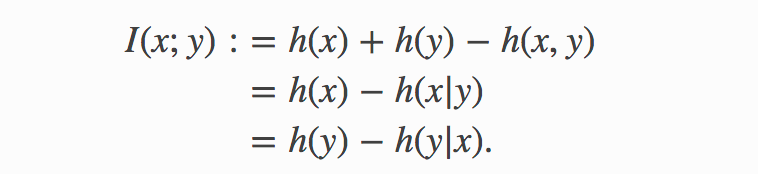
Fortunately, notions of informativeness and association are fully formalized by Information Theory. You’ll find a gentle primer on information theory here. For the purpose of this article, if we denote h(z) the entropy of a random variable — differential for continuous variable and Shannon for categorical variables, it suffices to recall that the canonical measure of how informative x is about y is their mutual information, defined as

幸運的是，信息性和關聯性的概念已被信息理論完全形式化。 您可以在這里找到有關信息論的入門文章。 出于本文的目的，如果我們表示h(z)的隨機變量的熵-連續變量的微分和分類變量的Shannon，則足以回想起x是y信息量的標準度量是它們的互信息，定義為

Some Key Properties of Mutual Information

互信息的一些關鍵屬性

The mutual information I(y; x) is well defined whether the output is categorical or continuous and whether inputs are continuous, categorical, or a combination of both. For some background reading on why this is the case, check out this primer and references therein.

很好地定義了互信息I(y; x)，無論輸出是分類的還是連續的，以及輸入是連續的，分類還是兩者的組合。 有關為什么會出現這種情況的一些背景知識，請查看此入門手冊和其中的參考文獻。

It is always non-negative and it is equal to 0 if and only if y and x are statistically independent (i.e. there is no relationship whatsoever between y and x).

當且僅當y和x在統計上獨立時(即y和x之間沒有任何關系)，它始終為非負且等于0 。

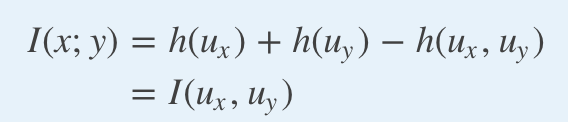
Additionally, the mutual information is invariant by lossless feature transformations. Indeed, if f and g are two one-to-one maps, then

另外，互信息通過無損特征變換而不變。 確實，如果f和g是兩個一對一的映射，則

A more general result, known as the Data Processing Inequality, states that transformations applied to x can only reduce its mutual information with y. Specifically,

更為普遍的結果稱為數據處理不等式 ，該結果表明，應用于x的轉換只能減少與y的互信息。 特別，

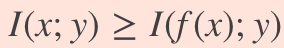
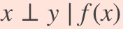
and the equality holds when f is either a one-to-one map, or y and x are statistically independent given f(x)

當f是一對一映射，或者y和x在給定f(x)時在統計上獨立時，等式成立

meaning that all the information about y that is contained in x is fully reflected in f(x) or, said differently, the transformation f preserves all the juice despite being lossy.

這意味著x中包含的有關y的所有信息都完全反映在f(x)中，或者換句話說，變換f盡管有損，但保留了所有汁液。

Thus, when mutual information is used as a proxy for quantifying the amount of juice in a dataset, effective feature engineering neither decreases nor increases the amount of juice, which is fairly intuitive. Feature engineering merely turns inputs and/or outputs into a representation that makes it easier to train a specific machine learning model.

因此，當將互信息用作量化數據集中果汁量的代理時，有效的特征工程既不會減少也不會增加果汁量，這非常直觀。 特征工程僅將輸入和/或輸出轉換為表示，使訓練特定機器學習模型變得更加容易。

From Mutual Information to Maximum Achievable Performance

從相互信息到最大可實現的績效

Although it reflects the essence of the amount of juice in a dataset, mutual information values, typically expressed in bits or nats, can hardly speak to a business analyst or decision-maker.

盡管它反映了數據集中果汁數量的本質，但是通常以位或小數表示的互信息值很難與業務分析師或決策者交流。

Fortunately, it can be used to calculate the highest performance that can be achieved when using x to predict y, for a variety of performance metrics (R2, RMSE, classification accuracy, log-likelihood per sample, etc.), which in turn can be translated into business outcomes. We provide a brief summary below, but you can find out more here.

幸運的是，對于各種性能指標(R2，RMSE，分類精度，每個樣本的對數似然性等)，它可以用于計算使用x預測y時可以達到的最高性能。轉化為業務成果。 我們在下面提供了一個簡短的摘要，但是您可以在此處找到更多信息 。

We consider a predictive model M with predictive probability

我們考慮具有預測概率的預測模型M

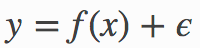
where f(x) is the model’s prediction for the output associated with inputs x. The model is a classifier when y is categorical and a regression model when y is continuous.

其中f(x)是模型對與輸入x關聯的輸出的預測。 當y為分類時，該模型為分類器；當y為連續時，該模型為回歸模型。

最大可達到R2 (Maximum Achievable R2)

In an additive regression model

在加性回歸模型中

the population version of the R2 is defined as

R2的人口版本定義為

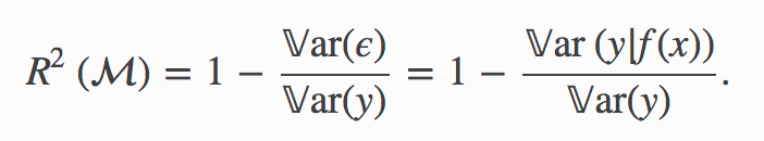
The ratio in the formula above represents the fraction of variance of the output that cannot be explained using inputs, under our model.

在我們的模型下，上式中的比率表示輸出方差的一部分，使用輸入無法解釋。

Although variance is as good a measure of uncertainty as it gets for Gaussian distributions, it is a weak measure of uncertainty for other distributions, unlike the entropy.

盡管方差像對高斯分布一樣是衡量不確定性的好方法，但與熵不同，對于其他分布而言，它是衡量不確定性的弱項。

Considering that the entropy (in nats) has the same unit/scale as the (natural) logarithm of the standard deviation, we generalize the R2 as follows:

考慮到熵 (以納特為單位 ) 與 標準偏差 的 (自然) 對數 具有相同的單位/標度 ，我們將R2概括如下：

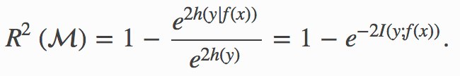
Note that when (y, f(x)) is jointly Gaussian (e.g. Gaussian Process regression, including linear regression with Gaussian additive noise), the information-adjusted R2 above is identical to the original R2.

注意，當(y，f(x))共同為高斯時(例如，高斯過程回歸，包括具有高斯累加噪聲的線性回歸)，上述信息調整后的R2與原始R2相同。

More generally, this information-adjusted R2 applies to both regression and classification, with continuous inputs, categorical inputs, or a combination of both.

更一般而言，此信息調整后的R2適用于回歸和分類，具有連續輸入，分類輸入或兩者的組合。

A direct application of the data processing inequality gives us the maximum R2 any model predicting y with x can achieve:

數據處理不平等的直接應用為我們提供了最大的R 2與X任何模型預測Y可以實現：

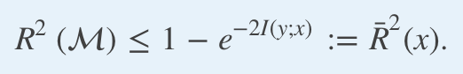
It is important to stress that this optimal R2 is not just an upper bound; it is achieved by any model whose predictive distribution is the true (data generating) conditional distribution p(y|x).

需要強調的是，這個最佳R2不僅僅是一個上限； 它可以通過任何預測分布為真實(數據生成)條件分布p(y | x)的模型來實現 。

最低可達到的RMSE (Minimum Achievable RMSE)

The population version of the Root Mean Square Error of the model above reads

上面模型的均方根誤差的總體版本為

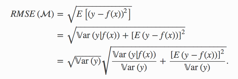
In the same vein, we may define its information-adjusted generalization as

同樣，我們可以將其信息調整后的概括定義為

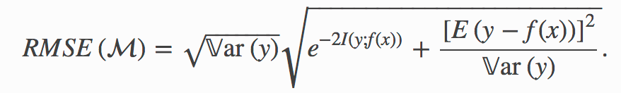
A direct application of the data processing inequality gives us the smallest RMSE any model using x to predict y can achieve:

數據處理不等式的直接應用為我們提供了最小的均方根誤差，任何使用x預測y的模型都可以實現：

最大可達到的真實對數似然 (Maximum Achievable True Log-Likelihood)

Similarly, the sample log-likelihood per observation of our model can be defined as

同樣，每次觀察模型的對數似然可定義為

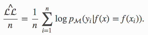
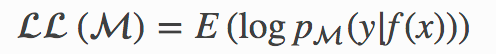
Its population equivalent, which we refer to as the true log-likelihood per observation, namely

它的總體當量，我們稱為每個觀察值的真實對數似然 ，即

satisfies the inequality

滿足不平等

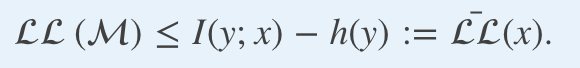
This inequality stems from the Gibbs and data processing inequalities. See here for more details.

這種不平等源于吉布斯和數據處理不平等。 有關更多詳細信息，請參見此處 。

Note that the inequality above holds true for both regression and classification problems and that the upper-bound is achieved— by a model using as its predictive distribution the true conditional p(y|x).

請注意，上述不等式對于回歸和分類問題均成立，并且通過使用真實條件p(y | x)作為其預測分布的模型實現了上限。

The term -h(y) represents the best true log-likelihood per observation that one can achieve without any data, and can be regarded as a naive log-likelihood benchmark, while the mutual information term I(y; x) represents the boost that can be attributed to our data.

-h(y)項表示每個觀察結果的最佳真實對數似然性，即無需任何數據即可獲得的觀測值，可以看作是幼稚的對數似然性基準，而互信息項I(y; x)則表示提升可以歸因于我們的數據。

最高可達到的分類精度 (Maximum Achievable Classification Accuracy)

In a classification problem where the output y can take up to q distinct values, it is also possible to express the highest classification accuracy that can be achieved by a model using x to predict y.

在輸出y可以占用q個不同值的分類問題中，還可能表示出最高的分類精度，這可以通過使用x預測y的模型來實現。

Let us consider the function

讓我們考慮一下功能

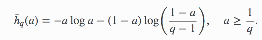
For a given entropy value h the best accuracy that can be achieved by predicting the outcome of any discrete distribution taking q distinct values, and that has entropy h is given by

對于給定的熵值h ，可以通過預測采用q個不同值的任何離散分布的結果獲得的最佳精度，并且具有熵h

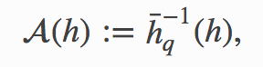
where the function

功能在哪里

is the inverse function of

是...的反函數

and is easily evaluated numerically. You can find more details here.

并且很容易用數字評估。 您可以在此處找到更多詳細信息。

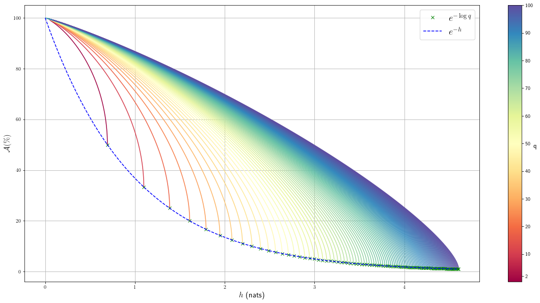
The figure below provides an illustration of the function above for various q.

下圖說明了上述各種q的函數。

More generally, the accuracy that can be achieved by a classification model M using x to predict a categorical output y taking q distinct values satisfies the inequality:

更一般而言，使用x預測帶有q個不同值的分類輸出y的分類模型M可以達到的精度滿足不等式：

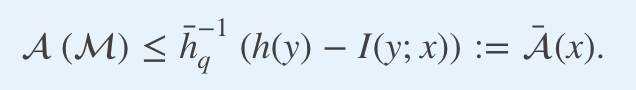
The entropy term h(y) reflects the accuracy of the naive strategy consisting of always predicting the most frequent outcome, namely

熵項h(y)反映了天真的策略的準確性，該策略包括始終預測最頻繁的結果，即

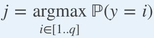
whereas the mutual information term I(y; x) accounts for the maximum amount of additional insights we can derive from our data.

而互信息項I(y; x)則說明了我們可以從數據中得出的最大附加見解量。

To sum-up, the highest value that can be achieved by virtually any population-based performance metric in a classification and regression problem can be expressed as a function of the mutual information of the true data generating distribution I(y; x) and a measure of the variability of the output (such as its entropy h(y), variance, or standard deviation) when the naive (inputs-less) predictive strategy does not have a null performance.

綜上所述，在分類和回歸問題中，幾乎任何基于人口的績效指標都可以實現的最高價值可以表示為真實數據生成分布的互信息的函數。 I(y; x)和輸出變異性的量度(例如其熵h(y) ，方差或標準偏差) 當幼稚(無輸入)預測策略沒有無效性能時。

Model-Free Mutual Information Estimation

無模型互信息估計

Finally, we can address the elephant in the room. Clearly it all boils down to estimating the mutual information I(y; x) under the true data generating distribution. However, we do not know the true joint distribution (y, x). If we knew it, we would have access to the best possible predictive model — the model with predictive distribution the true conditional p(y|x)!

最后，我們可以向房間里的大象講話。 顯然，這全都歸結為估計真實數據生成分布下的互信息I(y; x) 。 但是，我們不知道真正的聯合分布(y，x) 。 如果知道這一點，我們將有可能使用最佳的預測模型-具有預測分布的模型為真實條件p(y | x) ！

Fortunately, we do not need to know or learn the true joint distribution (y, x); this is where the inductive reasoning approach we previously mentioned comes into play.

幸運的是，我們不需要知道或學習真實的聯合分布(y，x) ； 這就是我們前面提到的歸納推理方法發揮作用的地方。

The inductive approach we adopt consists of measuring a wide enough range of properties of the data that indirectly reveal the structure/patterns therein, and infer the mutual information that is consistent with the observed properties, without making any additional arbitrary assumptions. The more flexible the properties we observe empirically, the more structure we will capture in the data, and the closer our estimation will be to the true mutual information.

我們采用的歸納方法包括測量足夠廣泛的數據屬性，這些屬性間接揭示其中的結構/模式，并推斷與觀察到的屬性一致的互信息，而無需進行任何其他任意假設。 我們憑經驗觀察到的屬性越靈活，我們將在數據中捕獲的結構越多，我們的估計就越接近真實的互信息。

To do so effectively, we rely on a few tricks.

為了有效地做到這一點，我們依靠一些技巧。

技巧I：在copula統一的雙重空間中工作。 (Trick I: Working in the copula-uniform dual space.)

First, we recall that the mutual information between y and x is invariant by one-to-one maps and, in particular, when y and x are ordinal, the mutual information between y and x is equal to the mutual information between their copula-uniform dual representations, defined by applying the probability integral transform to each coordinate.

首先，我們回想一下y和x之間的互信息是一對一映射不變的，尤其是當y和x為序數時， y和x之間的互信息等于它們的copula-之間的互信息。 統一對偶表示形式 ，通過將概率積分變換應用于每個坐標來定義。

Instead of estimating the mutual information between y and x directly, we estimate the mutual information between their copula-uniform dual representations; we refer to this as working in the copula-uniform dual space.

我們不是直接估計y和x之間的互信息，而是估計它們的copula-一致對偶表示之間的互信息。 我們稱其為在copula均勻雙空間中工作 。

This allows us to completely bypass marginal distributions, and perform inference in a unit/scale/representation-free fashion — in the dual space, all marginal distributions are uniform on [0,1]!

這使我們能夠完全繞過邊際分布，并以單位/比例/無表示的方式進行推理—在對偶空間中，所有邊際分布在[0,1]上都是均勻的！

技巧二：通過成對的斯皮爾曼等級關聯揭示模式。 (Trick II: Revealing patterns through pairwise Spearman rank correlations.)

We reveal structures in our data by estimating all pairwise Spearman rank correlations in the primal space, defined for two ordinal scalars x and y as

我們通過估計原始空間中所有成對的Spearman秩相關來揭示數據中的結構，原始空間針對兩個有序標量x和y定義為

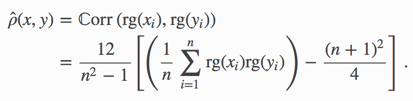
It measures the propensity for two variables to be monotonically related. Its population version is solely a function of the copula-uniform dual representations u and v of x and y and reads

它測量兩個變量單調相關的傾向。 它的總體版本僅是x和y的對數一致對偶表示u和v的函數 ，并且讀數為

In other words, using Spearman’s rank correlation, we may work in the dual space (a.ka. trick I) while efficiently estimating properties of interest in the primal space.

換句話說，使用Spearman的秩相關，我們可以在對偶空間(也稱為技巧I)中進行工作，同時有效地估計原始空間中感興趣的屬性。

Without this trick, we would need to estimate marginal CDFs and explicitly apply the probability integral transform to inputs to be able to work in the dual space, which would defeat the purpose of the first trick.

如果沒有這個技巧，我們將需要估計邊際CDF，并明確地將概率積分變換應用于輸入，以便能夠在對偶空間中工作，這將使第一個技巧的目的無效。

After all, given that the mutual information between two variables does not depend on their marginal distributions, it would be a shame to have to estimate marginal distributions to calculate it.

畢竟，鑒于兩個變量之間的相互信息不取決于其邊際分布，因此必須估算邊際分布以進行計算將是一個可恥的事情。

技巧三：擴展輸入空間以捕獲非單調模式。 (Trick III: Expanding the inputs space to capture non-monotonic patterns.)

Pairwise Spearman rank correlations fully capture patterns of the type ‘the output decreases/increases with certain inputs’ for regression problems, and ‘we can tell whether a bit of the encoded output is 0 or 1 based whether certain inputs take large or small values’ for classification problems.

成對的Spearman秩相關可完全捕獲類型“回歸時輸出降低/某些輸入增加”的模式，并且“我們可以根據某些輸入取大還是小來判斷編碼輸出的位是0還是1”用于分類問題。

To capture patterns beyond these types of monotonic associations, we need to resort to another trick. We note that, for any function f that is not injective, we have

要捕獲超出這些類型的單調關聯的模式，我們需要訴諸另一個技巧。 我們注意到，對于任何非內射函數f ，我們都有

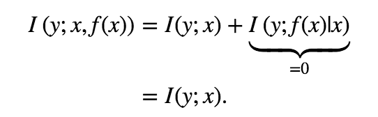
Thus, instead of estimating I(y; x), we may estimate I(y; x, f(x)) for any injective function f.

因此，代替估計I(y； x) ，我們可以估計任何內射函數f的 I(y； x，f(x)) 。

While pairwise Spearman rank correlations between y and x reveal monotonic relationships between y and x, f can be chosen so that pairwise Spearman correlations between y and f(x) capture a range of additional non-monotonic relationships between y and x.

而y和x之間的成對Spearman等級相關性揭示y和x之間的關系單調，f可以被選擇為使得y和F(X)之間的成對Spearman相關捕獲范圍的y和x之間的附加非單調關系。

A good example of f is the function

f的一個很好的例子是函數

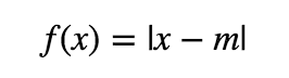
where m can be chosen to be the sample mean, median, or mode.

其中m可以選擇為樣本均值，中位數或眾數。

Indeed, if y = x2 for some mean zero and skew zero random variable x, then the Spearman rank correlation between y and x, which can be found to be 0 by symmetry, fails to reveal the structure in the data. On the other hand, the Spearman rank correlation between y and f(x) (with m=0), which is 1, better reflects how informative x is about y.

事實上，如果y = X 2為一些均值為零，歪斜零隨機變量x，那么y和x之間的Spearman等級相關性，這可以被認為是0由對稱性，未能揭示結構中的數據。 另一方面，Spearman等級之間的相關性 ? f(x) (其中m = 0 )為1 ，可以更好地反映x的信息量與y的關系 。

This choice of f captures patterns of the type ‘the output tends to decrease/increase as an input departs from a canonical value’. Many more types of patterns can be captured by using the same trick, including periodicity/seasonality, etc.

f的這種選擇捕獲了以下類型的模式：“當輸入偏離規范值時，輸出趨于減少/增加”。 通過使用相同的技巧，可以捕獲更多類型的模式，包括周期性/季節性等。

技巧四：使用最大熵原理將所有內容放在一起，以避免任意假設。 (Trick IV: Putting everything together using the maximum entropy principle as a way of avoiding arbitrary assumptions.)

To summarize, we define z=(x, f(x)), and we estimate the Spearman rank auto-correlation matrix of the vector (y, z), namely S(y, z).

總而言之，我們定義z =(x，f(x)) ，并估計向量(y，z)的Spearman等級自相關矩陣，即S(y，z)。

We then use as the density of the copula-uniform representation of (y, z) the copula density that, among all copula densities matching the patterns observed through the Spearman rank auto-correlation matrix S(y, z), has the highest entropy — i.e. the most uncertain about every pattern but the patterns observed through S(y, z).

然后，我們使用與在通過Spearman等級自相關矩陣S(y，z)觀察到的模式匹配的所有copula密度中具有最高熵的copula密度作為(y，z)的copula統一表示的密度。 —即除了通過S(y，z)觀察到的模式以外，每個模式中最不確定的部分。

Assuming (y, z) is d-dimensional, the resulting variational optimization problem reads:

假設(y，z)是d維的，則得出的變分優化問題為：

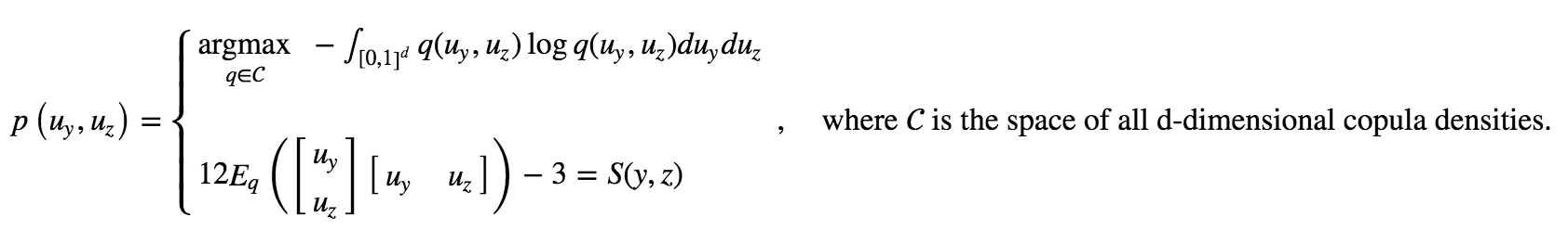
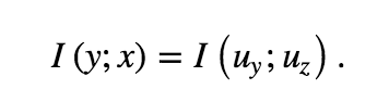
We then use the learned joint pdf to estimate the needed mutual information as

然后，我們使用學習的聯合pdf估計所需的互信息，如下

Making Sense of The Maximum-Entropy Variational Problem

認識最大熵變分問題

In the absence of the Spearman rank correlation constraints, the solution to the maximum-entropy problem above is the pdf of the standard uniform distribution, which corresponds to assuming that y and x are statistically independent, and have 0 mutual information. This makes intuitive sense, as we have no reason to believe x is informative about y until we gather empirical evidence.

在沒有Spearman秩相關約束的情況下，上述最大熵問題的解決方案是標準均勻分布的pdf，它對應于假設y和x在統計上獨立，并且具有0個互信息。 這是直覺上的意義，因為在收集經驗證據之前，我們沒有理由相信x對y具有信息意義。

When we observe S(y, z), the new solution to the variational maximum-entropy problem deviates from the uniform distribution just enough to reflect the patterns captured by S(y, z). Hence, our approach should not be expected to overestimate the true mutual information I(y; x).

當我們觀察到S(y，z)時 ，新的變分最大熵問題解決方案偏離了均勻分布，恰好足以反映S(y，z)捕獲的模式。 因此，不應期望我們的方法高估了真實的互信息I(y; x) 。

Additionally, so long as S(y, z) is expressive enough, which we can control through the choice of the function f, all types of patterns will be reflected in S(y, z), and our estimated mutual information should not be expected to underestimate the true mutual information I(y; x).2

另外，只要S(y，z)具有足夠的表現力(可以通過選擇函數f進行控制) ，所有類型的模式都將反映在S(y，z)中 ，而我們估計的互信息不應期望會低估真實的互信息I(y; x) .2

Application To An Ongoing Kaggle Competition

申請進行中的Kaggle比賽

We built the KxY platform, and the accompanying open-source python package to help organizations of all sizes cut down the risk and cost of their AI projects by focusing on high ROI projects and experiments. Of particular interest is the implementation of the approach described in this post to quantify the amount of juice in your data.

我們構建了KxY平臺以及隨附的開源python軟件包 ，通過專注于高ROI項目和實驗來幫助各種規模的組織降低其AI項目的風險和成本。 特別有趣的是實現本文中描述的方法以量化數據中的果汁量。

The kxy package can be installed from PyPi (pip install kxy) or Github and is also accessible through our pre-configured Docker image on DockerHub — for more details on how to get started, read this. Once installed, the kxy package requires an API key to run. You can request one by filling up our contact form, or by emailing us at demo@kxy.ai.

該KXY包可以從PyPI將被安裝(PIP安裝KXY)或Github上，也是通過我們的預配置上DockerHub泊塢窗圖像訪問-關于如何開始的詳細信息，請閱讀此 。 安裝后， kxy軟件包需要運行API密鑰。 您可以填寫我們的聯系表或通過電子郵件給我們，電子郵件為demo@kxy.ai。

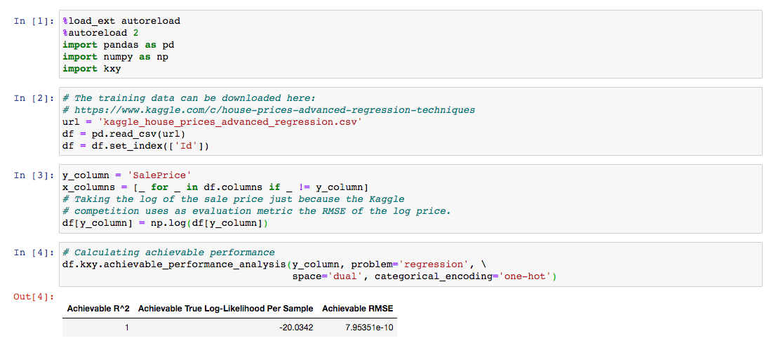
We use the House Price Advanced Regression Techniques Kaggle competition as an example. The problem consists of predicting house sale prices using a comprehensive list of 79 explanatory variables of which 43 are categorical and 36 are ordinal.

我們以房價高級回歸技術 Kaggle競賽為例。 問題在于使用79個解釋變量的綜合列表來預測房屋售價，其中43個是分類變量，36個是序數變量。

We find that when the one-hot encoding method is used to represent categorical variables, a near-perfect prediction can be achieved.

我們發現，當使用一熱編碼方法來表示分類變量時，可以實現近乎完美的預測。

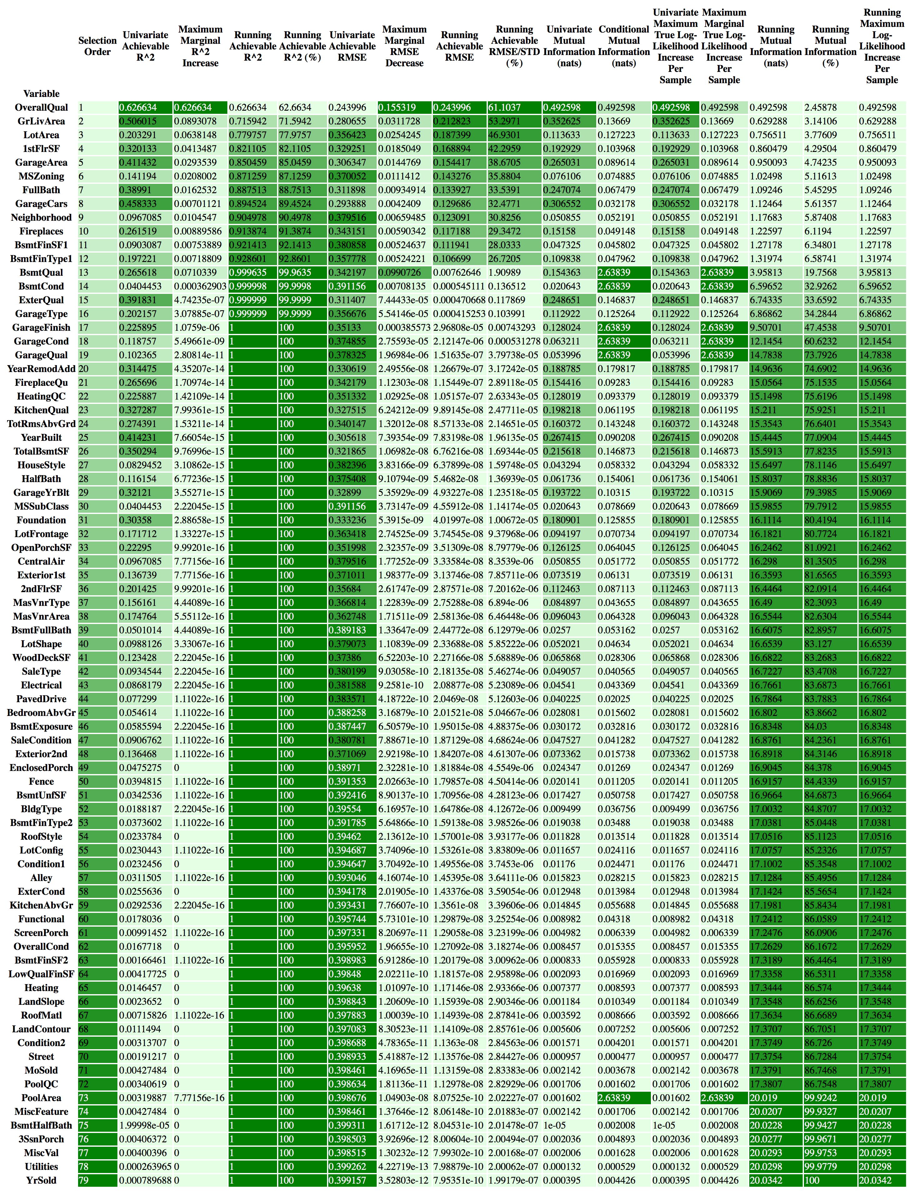
In fact, when we select explanatory variables one at a time in a greedy fashion, always choosing the variable that generates the highest amount of incremental juice among the ones that haven’t yet been selected, we find that with only 17 out of the 79 variables, we can achieve near-perfect prediction — in the R2 sense.

實際上，當我們一次貪婪地選擇一個解釋變量時，總是選擇在尚未選擇的變量中產生最大增量汁的變量，我們發現在79個變量中只有17個變量，我們可以實現接近完美的預測-在R2的意義上。

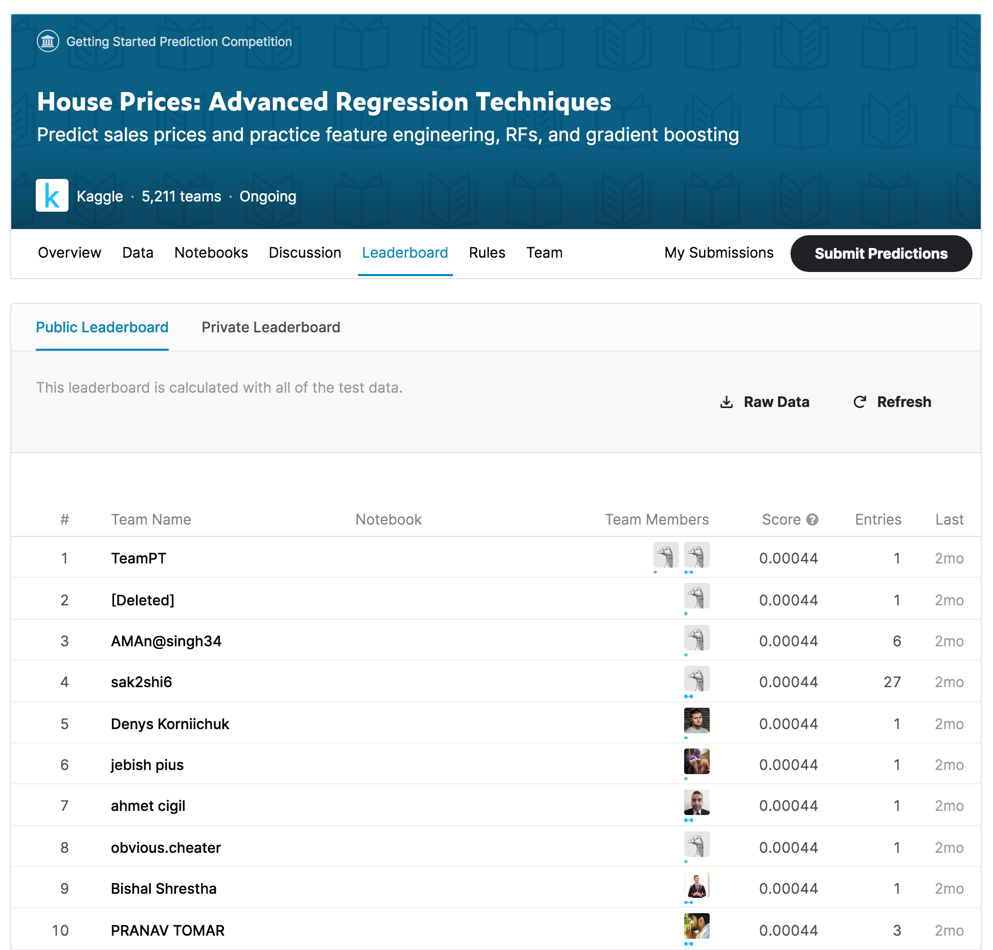
The figure below illustrates the result of the full variable selection analysis. Interestingly, the top of the current Kaggle leaderboard has managed to generate an RMSE of 0.00044, which is somewhere between the best that can be done using the top 15 variables, and the best that can be done using the top 16 variables.

下圖說明了完整變量選擇分析的結果。 有趣的是，當前Kaggle排行榜的頂部已成功生成0.00044的RMSE，介于使用前15個變量可以實現的最佳效果和使用前16個變量可以實現的最佳效果之間。

You’ll find the code used to generate the results above as a Jupyter notebook here.

在此處 ，您可以在Jupyter筆記本中找到用于生成結果的代碼。

Footnotes:

腳注：

[1] It is assumed that observations (inputs, output) can be regarded as independent draws from the same random variable (y, x). In particular, the problem should either not exhibit any temporal dependency or observations (inputs, output) should be regarded as samples from a stationary and ergodic time series, in which case your sample size should be long enough to span multiple of the systems’ memory.

[1]假設觀察值(輸入，輸出)可以視為來自同一隨機變量(y，x)的獨立繪制。 尤其是，問題應該不表現出任何時間依賴性，或者觀察值(輸入，輸出)應被視為來自平穩和遍歷時間序列的樣本，在這種情況下，樣本量應足夠長以覆蓋系統內存的倍數。

[2] The requirements of the previous footnote have very practical implications. The whole inference pipeline relies on the accurate estimation of the Spearman rank correlation matrix S(y, z). When observations can be regarded as i.i.d. samples, reliable estimation of S(y, z) only requires a small sample size and is indicative of the true latent phenomenon. On the other hand, when observations exhibit temporal dependency, if estimating S(y, z) using disjoint subsets of our data yields very different values, then the time series is either not stationary and ergodic or it is stationary and ergodic but we do not have a long enough history to characterize S(y, z); either way, the estimated S(y, z) will not accurately characterize the true latent phenomenon and the analysis should not be applied.

[2]上一個腳注的要求具有非常實際的意義。 整個推理流程依賴于Spearman秩相關矩陣S(y，z)的準確估計。 當觀測值可被視為同義樣本時，對S(y，z)的可靠估計僅需較小的樣本量，即可指示出真正的潛在現象。 另一方面，當觀測值表現出時間依賴性時，如果使用我們數據的不相交子集來估計S(y，z)會產生非常不同的值，則時間序列不是固定的和遍歷的，而是固定的和遍歷的，但我們不是具有足夠長的歷史來表征S(y，z); 無論哪種方式，估計的S(y，z)都無法準確地表征真實的潛在現象，因此不應進行分析。