This article is for those dummies like me, who’ve never tried to know what machine learning was or have left it halfway for the sole reason of being overwhelmed. Follow through every line and stay along. I promise you’d be quite acquainted with giving yourself your first project on your resume.

?他的文章是為那些傻瓜像我一樣，誰從來沒有試過才知道什么機器學習是或已經離開它對于中途被淹沒的唯一原因。 遵循每一條線并保持下去。 我保證您會非常熟悉在簡歷上給自己的第一個項目。

基本要領 (Basic Essentials)

We’d be doing the whole project in Python. The only essential is for you to understand basic programming. Nothing else is required. I prefer using Jupyter Notebook as an IDE as it helps in visualizing easier.

我們將用Python完成整個項目。 唯一的必要條件是您了解基本編程。 沒有其他要求。 我更喜歡將Jupyter Notebook用作IDE，因為它有助于簡化可視化過程。

介紹 (Introduction)

In this project, we shall make it interesting by using the data of the newly released Amazon Echo. Various customers who’ve bought the new Amazon Echo have submitted their reviews. We aim to predict whether a given review is positive or negative, through sentiment analysis. Sounds cool right? We shall use a dataset from Kaggle developed by Manu Siddhartha.

在這個項目中，我們將使用新發布的Amazon Echo的數據來使其有趣。 購買了新的Amazon Echo的各種客戶都提交了評論。 我們旨在通過情感分析來預測給定的評論是正面還是負面。 聽起來不錯吧？ 我們將使用Manu Siddhartha開發的Kaggle的數據集。

導入庫 (Importing Libraries)

Your first step is to import libraries. Libraries help us in increased functionality and reduce the bulkiness of the code. Type this into your first cell and press shift+enter.

第一步是導入庫。 庫可以幫助我們增加功能并減少代碼的龐大性。 在您的第一個單元格中鍵入內容，然后按shift + enter 。

1. Pandas is a software library written for python. We shall use it for data manipulation and make our calculations easier.

   Pandas是為python編寫的軟件庫。 我們將使用它進行數據處理，并使我們的計算更加容易。

2. NumPy is a high-performance library which we shall use to perform functions on the datasets and array.

   NumPy是一個高性能的庫，我們將使用它來對數據集和數組執行功能。

3. Seaborn and Matplotlib are visualization libraries. They help in providing insane visualizations where we shall derive our insights.

   Seaborn和Matplotlib是可視化庫。 它們有助于提供瘋狂的可視化效果，從中我們可以得出自己的見解。

When we say ‘as’ in the code above, we imply that the name of the library shall be called as the text mentioned, for ease of effort.

當我們在上面的代碼中用“ as”表示時，我們的意思是為了方便起見，庫的名稱應稱為所提到的文本。

導入數據集 (Importing Dataset)

We shall use a Kaggle dataset. Use the link below to download the dataset into your project folder.

我們將使用Kaggle數據集。 使用下面的鏈接將數據集下載到您的項目文件夾中。

After you download, type the following and press shift+enter to import the dataset.

下載后，鍵入以下內容，然后按shift + enter導入數據集。

echo = pd.read_csv(‘amazon_alexa.tsv’,sep=’\t’)

echo = pd.read_csv('amazon_alexa.tsv'，sep ='\ t')

1. echo =: We assign the dataset to variable named echo

   echo =：我們將數據集分配給名為echo的變量

2. sep=’\t’: The dataset contains values separated by a tab ( tsv files ).We use the sep argument to mention the separation.

   sep ='\ t'：數據集包含由制表符分隔的值(tsv文件)。我們使用sep參數來提及分隔。

3. ‘amazon_alexa.tsv’: If the file is in any other place than the Jupyter Notebook folder, mention the path of the file followed by /amazon_alexa.tsv inside the quotes.

   'amazon_alexa.tsv'：如果文件位于Jupyter Notebook文件夾以外的任何其他位置，請在引號中提及文件的路徑，后跟/amazon_alexa.tsv 。

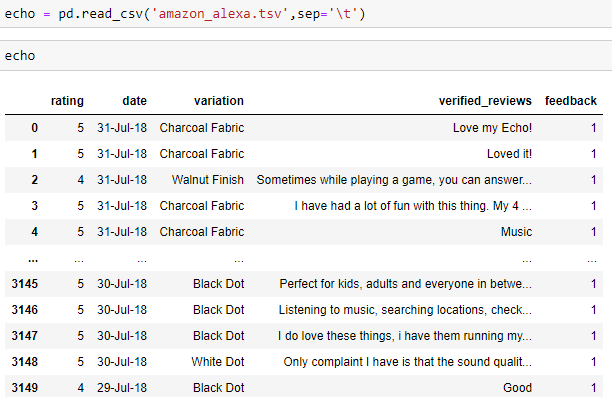
Type echo in the cell below and you shall see the dataset you’ve imported.

在下面的單元格中鍵入echo，您將看到導入的數據集。

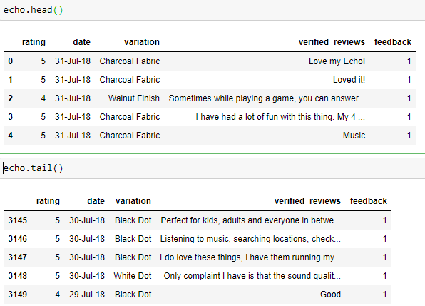
The dataset consists of the rating given, date of review, model variation, the reviews that the customers have written, and the feedback. Here, 1=positive and 0=negative. The column feedback shall be our target.

數據集包括給定的評級，審查日期，模型變化，客戶撰寫的審查以及反饋。 在此，1 ＝正，0 ＝負。 列反饋將是我們的目標。

查看您的數據集 (Viewing your dataset)

Technical information on your dataset is essential as it helps us understand what we’re dealing with. Use the following codes in the images below.

您的數據集上的技術信息至關重要，因為它可以幫助我們了解我們正在處理的內容。 在下面的圖像中使用以下代碼。

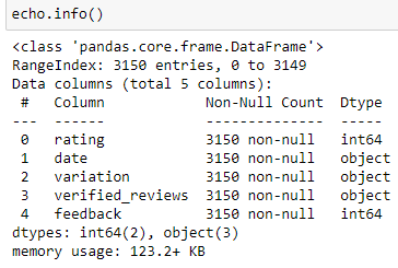
1. echo.info(): Gives us information on the null values and non-null values in the dataset. It mentions the datatype of the column

   echo.info()：為我們提供有關數據集中的空值和非空值的信息。 它提到了列的數據類型

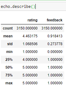
2. echo.describe(): Given us information about the column’s average, count, mean and a lot of other mathematical deductions

   echo.describe()：為我們提供有關列的平均值，計數，均值和許多其他數學推論的信息

3. .head() and .tail() : Display us the first 5 and the last 5 rows of the dataset respectively. .head(n) where n is the number of rows you’d want to display. The same applies to a tail too.

   .head()和.tail()：分別顯示數據集的前5行和后5行。 .head(n) ，其中n是您要顯示的行數。 尾巴也是如此。

數據可視化 (Data Visualization)

Visualizing the data in a given dataset remains unique to each as the conclusions we draw and the opinion we generate would differ. But for the purpose to learn, let’s look at a few examples and explore the dataset. Each visualization shall have the code at the top. And I shall explain the code in detail, as it’d make it easier the next time to create your visualizations.

可視化給定數據集中的數據對于每個數據集仍然是唯一的，因為我們得出的結論和產生的觀點會有所不同。 但是出于學習的目的，讓我們看一些示例并探索數據集。 每個可視化文件的頂部均應具有代碼。 我將詳細解釋代碼，因為這將使下一次創建可視化文件變得更加容易。

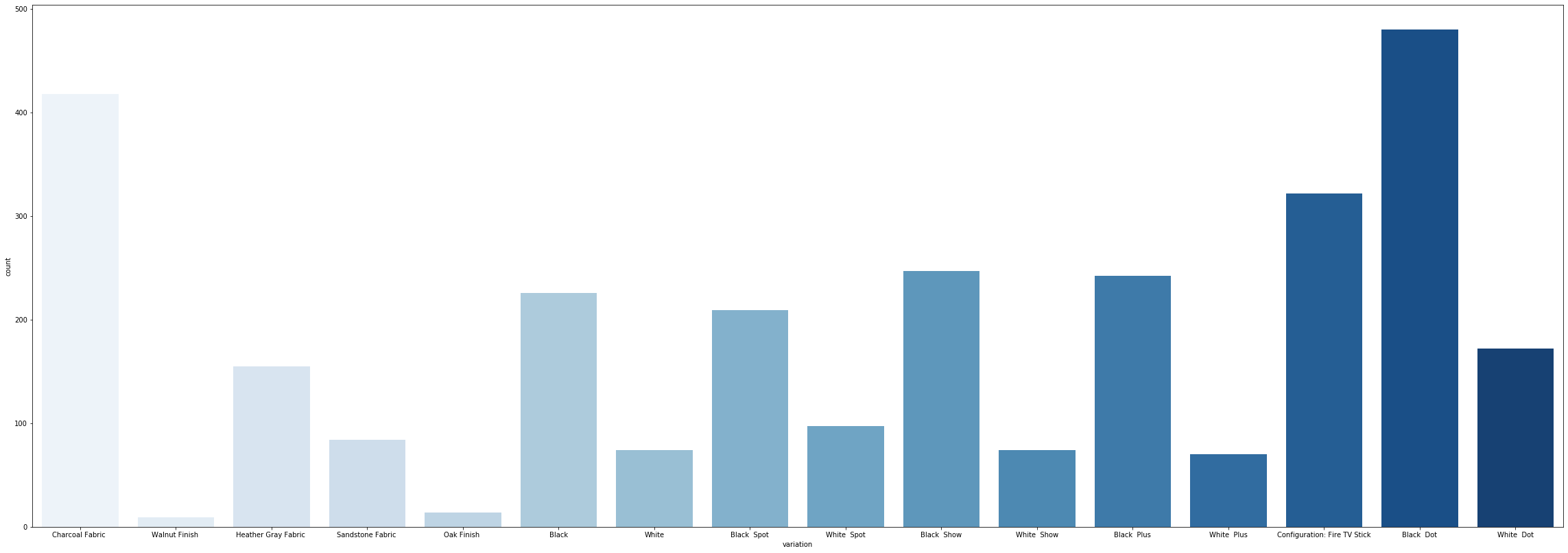
每個型號的審查數量 (Review count for each model variant)

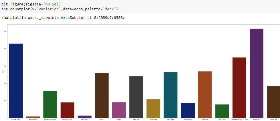
1. plt.figure(figsize=[40,14]) = Helps us in setting the dimensions of the image. 40,14 implies that the breadth shall be 40 units and the height shall be 14 units respective to scale.

   plt.figure(figsize = [40,14])=幫助我們設置圖像的尺寸。 40,14表示寬度應為40個單位，高度應為14個單位(按比例)。

2. sns.countplot(x=’variation’,data=echo,palette=’dark’) = countplot show us the count of each section on the x axis. palette = ‘dark’ is a color palette we would want our visualizations to be in.

   sns.countplot(x ='variation'，data = echo，palette ='dark')= countplot向我們展示x軸上每個部分的計數。 Palette ='dark'是我們希望可視化效果出現的調色板。

Some of the inferences that we could assume would be that, the variant Black Dot has the highest amount of reviews and the Walnut Fresh has the lowest amount of reviews. Assumptions could follow that the Black dot was purchased the most and the Walnut fresh the least.

我們可以假設的一些推論是，變體黑點的評論量最高，而核桃新鮮的評論量最低。 可以假設購買了最多的黑點，而購買了最少的核桃。

評級多數 (Rating Majority)

To understand the count of ratings that people have given we can generate a histogram. In the aforesaid image, we can deduce that majority of the people have given it a 5-star rating which can assure us product success. No product is perfect and obviously, we are going to have lower ratings too.

要了解人們給予的評分數量，我們可以生成直方圖。 在上述圖像中，我們可以推斷出大多數人給它的5星評級可以確保我們的產品成功。 沒有產品是完美的，顯然，我們也將獲得更低的評分。

.hist(bins=n) : It generates a histogram where bins is the measure of the average distancing and range. You are free to explore placing numbers of your choice for varied graphs.

.hist(bins = n)：它生成一個直方圖，其中bins是平均距離和范圍的度量。 您可以自由探索各種圖形的放置編號。

正面和負面評論 (Positive & Negative Reviews)

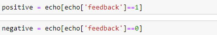
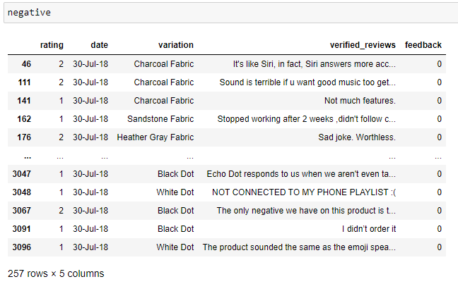
Now that we’ve had a basic overview, let’s get down to analyzing positive and negative reviews. To generate all the rows which contain both positive and negative reviews do the following.

現在我們已經有了基本概述，讓我們開始分析正面和負面評論。 要生成同時包含正面和負面評論的所有行，請執行以下操作。

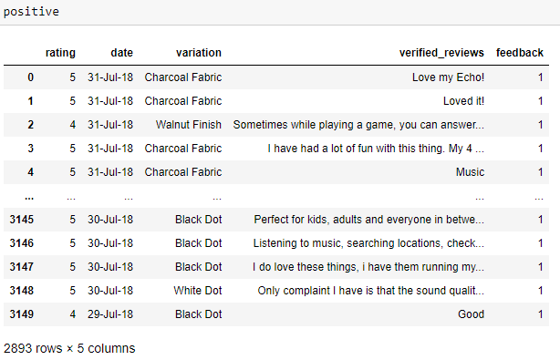
This shall store all the respective positive and negative reviews into the respective variables. To display the tables just type in the name of the variable into a new cell. The following shall be displayed.

這會將所有各自的正面和負面評論存儲到各自的變量中。 要顯示表，只需在新單元格中鍵入變量名稱即可。 將顯示以下內容。

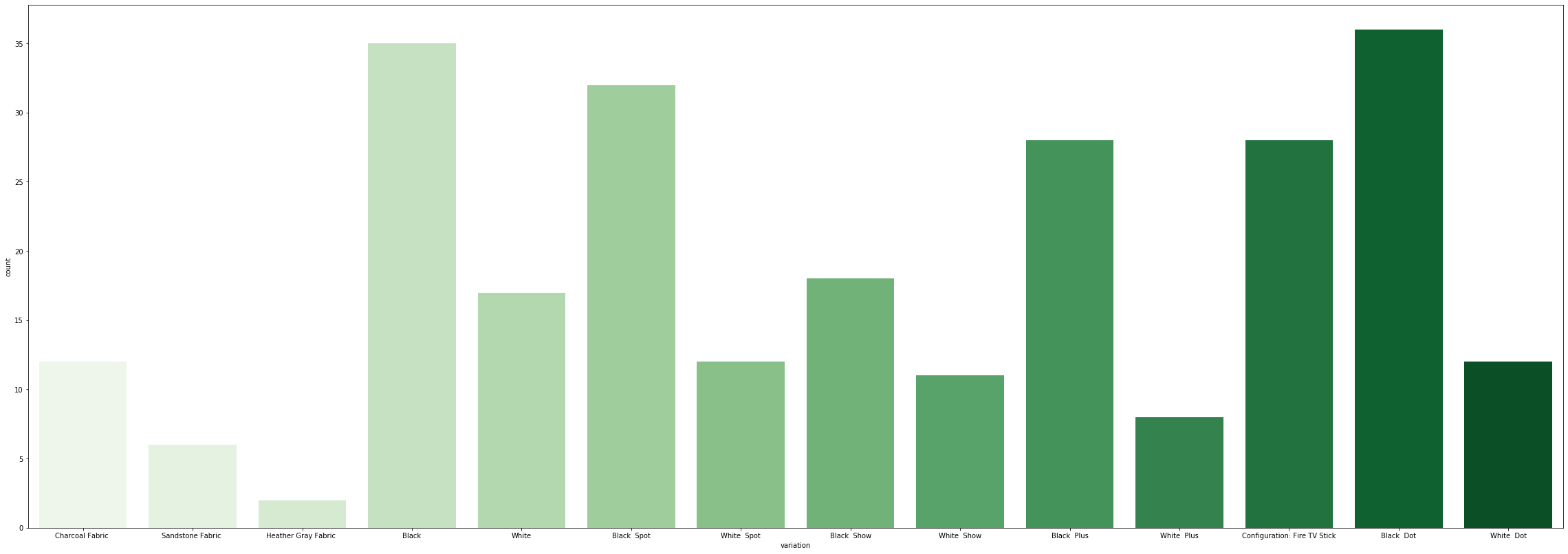
負反饋計數wrt。 變異 (Negative feedback count wrt. variation)

The following set of codes shall depict us the count-plots of both positive and negative feedbacks with respect to different variants.

以下代碼集將向我們描述有關不同變體的正反饋和負反饋的計數圖。

plt.figure(figsize=[40,14])sns.countplot(x=’variation’,data=positive,palette=’Blues’)

plt.figure(figsize = [40,14])sns.countplot(x ='variation'，data = positive，palette ='Blues')

plt.figure(figsize=[40,14])sns.countplot(x=’variation’,data=negative,palette=’Greens’)

plt.figure(figsize = [40,14])sns.countplot(x ='variation'，data = negative，palette ='Greens')

特征工程 (Feature Engineering)

Feature Engineering plays a vital role in developing the right model. We can improve the performance of machine learning algorithms. Amongst the numerous steps of feature engineering, we shall concentrate on a few major steps which shall help us in developing our model.

功能工程在開發正確的模型中起著至關重要的作用。 我們可以提高機器學習算法的性能。 在特征工程的眾多步驟中，我們將集中于幾個主要步驟，這些步驟將有助于我們開發模型。

驅逐不必要的數據 (Evicting unnecessary data)

Our first step is to drop those columns which we think shall be unnecessary in deriving whether the reviews are positive or negative. You are free to experiment with the columns you like. But here’s what I’ve deduced. So let us have a look at all the columns we’ve got.

我們的第一步是刪除那些我們認為在得出正面或負面評論時不必要的列。 您可以隨意嘗試自己喜歡的列。 但是，這就是我的推論。 因此，讓我們看看我們擁有的所有列。

1. Rating: Important to know how well the customer likes the product. The review and the rating are majorly directly proportional to each other.

   評分：了解客戶對產品的滿意程度很重要。 評論和評分主要是直接成比例的。

2. Variation: The model variant shall play an important role in because there might be opinions the color too.

   變體：模型變體在其中起著重要作用，因為可能還會有顏色的意見。

3. Date: Not necessary. It has nothing to do with the emotion o the review.

   日期：不需要。 它與評論的情感無關。

4. Verified Reviews: Obviously Needed!

   驗證評論：顯然需要！

5. Feedback: Bah! Our target Column. We need it.

   反饋：B ！ 我們的目標專欄。 我們需要。

So to eliminate the date column use the following code. This shall remove the column ‘date’ from the dataset.

因此，要消除日期列，請使用以下代碼。 這將從數據集中刪除“日期”列。

echo.drop(‘date’,axis=1,inplace=True)

echo.drop('date'，axis = 1，inplace = True)

1. inplace=True: inplace is generally used for two cases. When we mention True, it removes the column permanently, and when False it displays us the dataset without the column only for that iteration. The next time you view your dataset, the column re-appears.

   inplace = True： inplace通常用于兩種情況。 當我們提到True時，它將永久刪除列，而當False時，它將向我們顯示不包含該迭代的數據集。 下次查看數據集時，該列會重新出現。

2. axis = 1 : ensures the column is removed vertically

   軸= 1：確保垂直卸下色譜柱

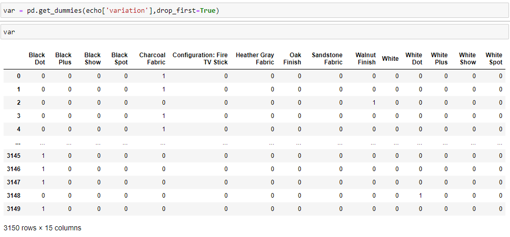
虛擬您的數據 (Dummy your data)

Imagine a huge table where one of the columns has only the values A, B, and C. In simple terms, a machine cannot understand these A, B, and C while we vectorize. So the cleverest way is to create 3 new additional columns A, B, and C and if that specific row contains the value, we shall mention binaries such as 1 or 0. This way we’ve depicted the value’s presence in the row. Neat?

想象一個巨大的表，其中的一列只有值A，B和C。簡單來說，當我們進行矢量化處理時，機器無法理解這些A，B和C。 因此，最聰明的方法是創建3個新的附加列A，B和C，如果該特定行包含該值，我們將提及諸如1或0之類的二進制文件。這種方式我們已經描述了該值在行中的存在。 整齊？

The same shall be applied to our dataset. We shall dummy our ‘variation’ column through the same procedure. It’s a simple 3 step process.

這同樣適用于我們的數據集。 我們將通過相同的程序來偽裝“變化”列。 這是一個簡單的三步過程。

var = pd.get_dummies(echo[‘variation’],drop_first=True)

var = pd.get_dummies(echo ['variation']，drop_first = True)

This creates a dataset with columns named after the variation names, whilst showing its presence through binaries.

這將創建一個數據集，其中包含以變體名稱命名的列，同時通過二進制文件顯示其存在。

The next obvious step shall be to merge this dataset to our main dataset. To do this let us type the following. And after we merge the datasets, it does not make any point to have the original column. So we shall drop the column.

下一步顯然是將這個數據集合并到我們的主要數據集中。 為此，我們鍵入以下內容。 合并數據集后，擁有原始列毫無意義。 因此，我們將刪除該列。

1. echo = pd.concat([echo,var],axis=1)

   echo = pd.concat([echo，var]，axis = 1)

2. echo.drop(‘variation’,axis=1,inplace=True)

   echo.drop('variation'，axis = 1，inplace = True)

最后步驟 (Last Steps)

We’re nearly there. All it takes is a few careful steps and understanding to get through. Now as I’ve mentioned earlier, the machine does not understand the text. The only column with text now is the reviews column. Here’s how we shall break it down. For example, if we have the first row as

我們快到了。 它所需要的只是一些謹慎的步驟和理解以實現。 現在，正如我之前提到的，機器不理解文本。 現在唯一帶有文本的列是評論列。 這是我們將其分解的方法。 例如，如果我們有第一行作為

row 1: The doughnut is amazing: 1

第1行：甜甜圈很棒：1

Our idea here is to generate, columns for every word in the text and update its count through binaries. Very similar to dummying, but different. So after applying the same to several rows, the column ‘THE’ might have various 1s and 0s. The logic behind this is that the machine understands the frequency of usage of words in a particular order to understand the sentiment. Not clear? Which word comes after what and it’s frequency is what the machine analyzes. This can be achieved through a few steps. Follow through.

我們的想法是為文本中的每個單詞生成列，并通過二進制更新其計數。 與虛擬非常相似，但有所不同。 因此，將其應用于多行之后，列“ THE”可能具有各種1和0。 其背后的邏輯是，機器以特定順序理解單詞使用的頻率以理解情緒。 不清楚？ 機器分析的內容是哪個單詞緊隨其后，它的出現頻率。 這可以通過幾個步驟來實現。 遵循。

1. In the first line, we are importing a CountVectorizer from the scikit-learn(sklearn) library

   在第一行中，我們從scikit-learn (sklearn)庫中導入CountVectorizer

2. We create an object — cv

   我們創建一個對象-cv

3. On the column verified_reviews in the echo dataset, we shall apply the cv.fit_transform function to create column counts for each word.

   在回顯數據集中的authenticated_reviews列上，我們將應用cv.fit_transform函數為每個單詞創建列數。

This stores all the transformed data into rows with counts. Our next step is to convert it into an array. Convert this array into a dataset. And then, merge it to the main dataset. The final step is to drop the column which had initially contained the reviews. Execute the following codes and the results should look something similar to this.

這會將所有轉換后的數據存儲到帶有計數的行中。 我們的下一步是將其轉換為數組。 將此數組轉換為數據集。 然后，將其合并到主數據集中。 最后一步是刪除最初包含評論的列。 執行以下代碼，結果應與此類似。

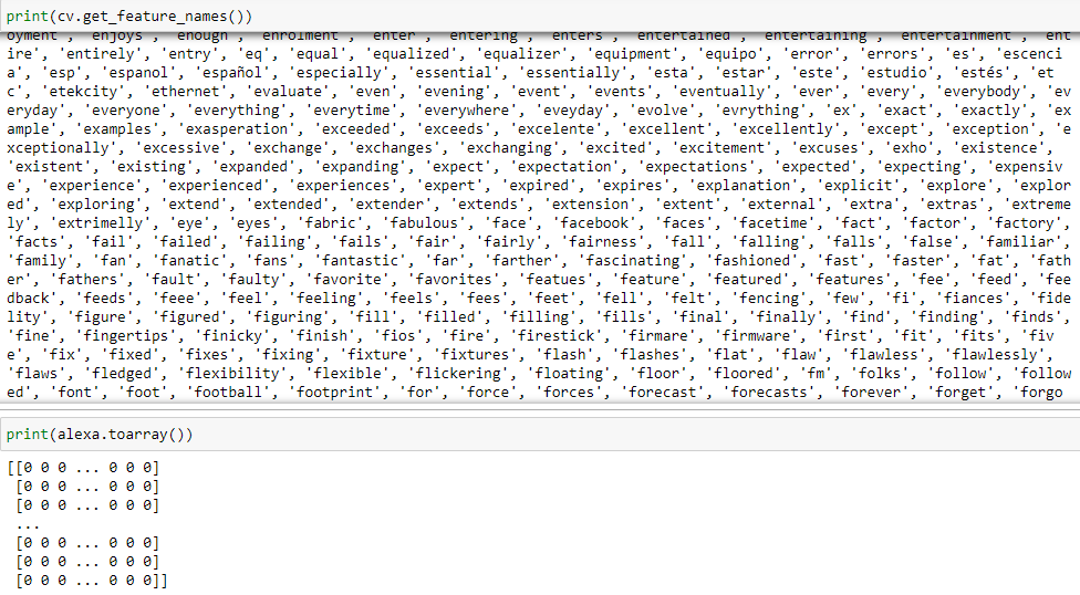
reviews = pd.DataFrame(alexa.toarray()): This piece of code sees to it that a new data frame is created with the counts of all individual words.

reviews = pd.DataFrame(alexa.toarray())：這段代碼可以看到它創建了一個帶有所有單個單詞計數的新數據框。

訓練數據 (Training your Data)

The first most important step in training your data is to divide the data into input and output. We shall consider the variable X to be our input and variable Y to be our output.

訓練數據的最重要的第一步是將數據分為輸入和輸出。 我們將變量X作為我們的輸入，并將變量Y作為我們的輸出。

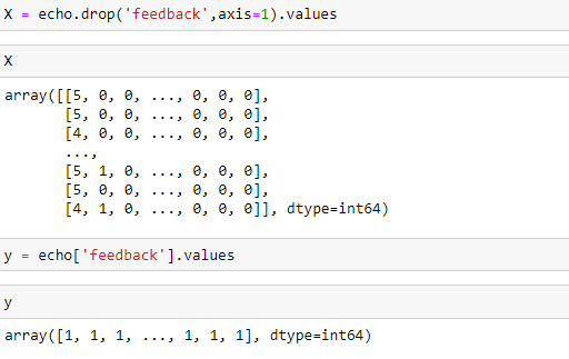
X shall contain all the columns except the feedback columns, because that’s what we have to predict

X應該包含除反饋列之外的所有列，因為這是我們必須預測的

Y shall contain the feedback column as it is our dataset.

Y應該包含反饋列，因為它是我們的數據集。

Our next step is to split the data into testing and training. To check the accuracy of how well we’ve predicted we shall split our dataset itself because the reviews are from the same origin. You can experiment by creating your testing dataset too, but this is to make things work faster. Type the following code.

我們的下一步是將數據分為測試和培訓。 為了檢查預測的準確性，我們將拆分數據集本身，因為評論來自同一來源。 您也可以通過創建測試數據集進行試驗，但這是為了使工作更快。 輸入以下代碼。

Now our data has split into input — training and testing, output — training and testing. test_size implies that we use 20% of the dataset as our testing dataset.

現在，我們的數據已分為輸入(培訓和測試)，輸出(培訓和測試)。 test_size表示我們使用數據集的20％作為測試數據集。

The final step is to apply an algorithm that shall vectorize all the input data into one and use it for training. We shall use a Random Forest Classifier to do this. Type the following code into your cells. The output should look something similar to this.

最后一步是應用一種算法，該算法應將所有輸入數據矢量化為一個并用于訓練。 我們將使用隨機森林分類器執行此操作。 在您的單元格中鍵入以下代碼。 輸出應類似于此。

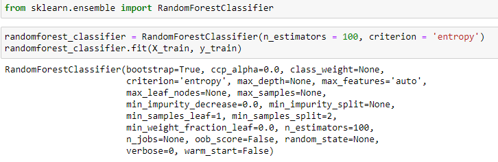
This step shall train your model completely and now your model is ready to go for testing if you’ve got something similar to this. Understanding the Random Forest Classifier algorithm is beyond the scope of the article. The easiest method to understand is as follows.

此步驟將完全訓練您的模型，如果您有類似的東西，現在您的模型已準備好進行測試。 了解隨機森林分類器算法超出了本文的范圍。 最容易理解的方法如下。

Given a set of inputs, the algorithms create n_estimators number of trees where each tree has a different combined connection where it trains itself amongst different iterations.

給定一組輸入，算法將創建 n_estimators 數量的樹，其中每棵樹具有不同的組合連接，并在不同的迭代中訓練自己。

Now that you’ve completed the penultimate step, let’s proceed to final step.

現在您已經完成了倒數第二步，讓我們繼續最后一步。

測試數據 (Testing your Data)

Remember how we’ve split our data into training and testing. It’s time to use our testing data. Type in the following code.

記住我們如何將數據分為訓練和測試。 現在該使用我們的測試數據了。 輸入以下代碼。

y_predict = randomforest_classifier.predict(X_test)

y_predict = randomforest_classifier.predict(X_test)

This assigns all the predicted values to the variable y_predict. Now our only step left is to visualize and check how well our model has performed. For this, We shall compare the predicted values in comparison to the original tested values. We shall import a classification report and a confusion matrix for this. These shall be explained in forthcoming articles. For now, let’s stick to analyzing them. Type the following code.

這會將所有預測值分配給變量y_predict 。 現在，我們剩下的唯一步驟就是可視化并檢查模型的性能。 為此，我們將比較預測值與原始測試值。 我們將為此導入分類報告和混淆矩陣。 這些將在以后的文章中進行解釋。 現在，讓我們繼續分析它們。 輸入以下代碼。

from sklearn.metrics import confusion_matrix,classification_report

從sklearn.metrics導入confusion_matrix，classification_report

38 : How many values have been accurately predicted.

38：已經準確預測了多少個值。

5.8e+02 : No. of false values have been predicted right.

5.8e + 02：正確預測的錯誤值數量。

9 : Suggests us the number of right values predicted wrong. (Type 1 error)

9：向我們建議預測錯誤的正確值的數量。 (類型1錯誤)

1 : The number of wrong ones predicted right. ( type 2 error )

1：預測正確的錯誤數目。 (類型2錯誤)

To finally predict accuracy and the precision type the following code.print(classification_report(y_test, y_predict))

要最終預測精度和精度，請鍵入以下代碼。 打印(classification_report(y_test，y_predict))

And there you go! Here’s to your first Machine Learning project.

然后你去了！ 這是您的第一個機器學習項目。

Nikhilesh Garnepudy

尼希列什·加內普迪(Nikhilesh Garnepudy)