前言 (Preface)

If you are reading this, it’s most likely because you love to solve puzzles. I’m a very competitive person by nature. The Mt. Everest of puzzles, in my opinion, is trying to find excess returns through active trading in the stock market. This blog is my first of many posts of an attempt to — hopefully — summit the intimidating Mt. Everest of algorithmic trading and emerge profitably.

如果您正在閱讀本文，則最有可能是因為您喜歡解決難題。 我天生就是一個很有競爭力的人。 山。 我認為，珠穆朗瑪的難題正試圖通過股票市場上的活躍交易來尋找超額收益。 這個博客是我嘗試(希望)登頂這座令人生畏的山峰的眾多文章中的第一篇。 算法交易的珠穆朗瑪峰并盈利。

First off, I must atone for my sins. I am a failed daytrader. I attempted day trading over a summer during a hiatus from work. Everything I read told me to have a plan before I entered a trade, and when I did enter a trade to stick to my trading plan despite whatever emotion I may be feeling. I was confident that this would be no problem. I have a pretty good grasp on all my vices — don’t we all? If you’re human, then the answer is no. No, you don’t have your vices under control. That is the literal definition of a vice. I was naive and thankfully was able to quit before I did any real damage to my account. However, like a moth to a flame, I can’t leave a good puzzle. I am going back into the fray, but this time I have a plan. I plan on building a purely quantitative system that removes the worst part of any trading plan (yourself) from the equation.

首先，我必須贖罪。 我的交易員失敗了。 我在工作中斷期間試圖在整個夏天進行日間交易。 我閱讀的所有內容都告訴我在進入交易之前要有一個計劃，而當我進入交易時要堅持我的交易計劃，盡管我可能會感到任何情緒。 我相信這不會有問題。 我對所有的惡習都掌握得很好–不是所有人嗎？ 如果您是人類，那么答案是否定的。 不，您不受控制。 那是惡習的字面定義。 我很天真，幸好我能夠在對帳戶造成任何實際損失之前退出。 但是，就像飛蛾撲火一樣，我不能留下一個好謎。 我將重返戰場，但是這次我有一個計劃。 我計劃建立一個純粹的量化系統，以消除等式中任何交易計劃(您自己)的最糟糕部分。

Before you go any farther, let me say this blog post is simply about ARIMA models, and this preface is just a teaser for the full algorithmic trading system that will come in the future. If the intro did not scare you off, let’s begin with a simple ARIMA model that helps us predict tomorrow’s daily closing price of whatever stock you choose.

在繼續之前，請允許我說這篇博客文章只是關于ARIMA模型的，并且此序言只是對將來將要使用的完整算法交易系統的預告。 如果介紹沒有嚇倒您，讓我們從一個簡單的ARIMA模型開始，該模型可以幫助我們預測所選股票的明天每日收盤價。

讓我們編碼 (Let’s Code)

ARIMA is an acronym that stands for AutoRegressive Integrated Moving Average. Throughout this blog, I will break down the steps necessary to implement a successful ARIMA model.

ARIMA是首字母縮寫詞，代表自動回歸綜合移動平均線。 在整個博客中，我將分解實現成功ARIMA模型的必要步驟。

步驟1：取得資料 (Step 1: Get the data)

For this example, we will use the SPY ETF. The SPY is an ETF that mimics the S&P500, which is a basket of stocks weighted by market cap. Many ETFs mimic the S&P 500, but this is the most common and most liquid fund.

在此示例中，我們將使用SPY ETF。 SPY是模仿S＆P500的ETF，S＆P500是按市值加權的一籃子股票。 許多ETF模仿標準普爾500指數，但這是最常見和最具流動性的基金。

To use this, we will use the yfinance API. If you do not have this API installed, a simple pip install in your Jupyter Notebook should do. If you wish to learn more about this API, check out the PyPI page for more details.

要使用此功能，我們將使用yfinance API。 如果您尚未安裝此API，則應該在Jupyter Notebook中進行簡單的pip安裝。 如果您想了解更多有關此API的信息， 請查看PyPI頁面以獲取更多詳細信息 。

!pip install yfinance

Now, let’s pull the entire daily history of the ticker “SPY” into a neat data frame.

現在，讓我們將股票代碼“ SPY”的整個每日歷史記錄拉入一個整潔的數據框中。

import yfinance as yf
import pandas as pdspy = yf.Ticker("SPY")# get stock info
spy.info# get historical market data as df
hist = spy.history(period="max")# Save df as CSV
hist.to_csv('SPY.csv')# Read back in as dataframe
spy = pd.read_csv('SPY.csv')# Convert Date column to datetime
spy['Date'] = pd.to_datetime(spy['Date'])

If you print out “spy.info” you will get a dictionary of a lot of extra data on the stock. All we are currently worried about for this model is the closing price. The object “hist” is a dataframe, and we send it to CSV to have a local copy. You can run this every day after the market closes and get the most up to date information if you want.

如果您打印出“ spy.info”，您將獲得有關大量庫存額外數據的詞典。 我們目前對此模型擔心的只是收盤價。 對象“ hist”是一個數據框，我們將其發送到CSV以獲取本地副本。 您可以在市場收盤后每天執行此操作，并根據需要獲取最新信息。

步驟2：分割資料 (Step 2: Split your data)

This code is coming directly from my notebook, which multiple models in it, so the data split may seem a bit overkill. For purely this ARIMA model, you would only need a train and test data set. However, the code I provide splits the data into a train, test, and validation data set. Splitting your data is extremely important in all machine learning applications.

這段代碼直接來自我的筆記本，筆記本中有多個模型，因此數據拆分似乎有些過頭。 僅對于此ARIMA模型，您只需要訓練和測試數據集。 但是，我提供的代碼將數據分為訓練，測試和驗證數據集。 在所有機器學習應用程序中，分割數據極為重要。

# Set target series
series = spy['Close']# Create train data set
train_split_date = '2014-12-31'
train_split_index = np.where(spy.Date == train_split_date)[0][0]
x_train = spy.loc[spy['Date'] <= train_split_date]['Close']# Create test data set
test_split_date = '2019-01-02'
test_split_index = np.where(spy.Date == test_split_date)[0][0]
x_test = spy.loc[spy['Date'] >= test_split_date]['Close']# Create valid data set
valid_split_index = (train_split_index.max(),test_split_index.min())
x_valid = spy.loc[(spy['Date'] < test_split_date) & (spy['Date'] > train_split_date)]['Close']#printed index values are: 
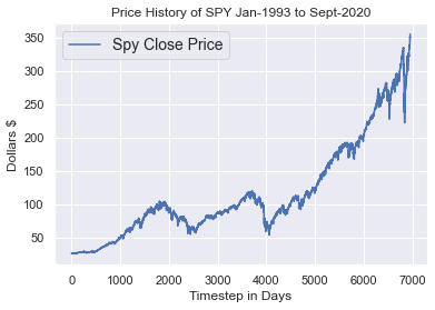
#0-5521(train), 5522-6527(valid), 6528-6947(test)

I chose these dates pretty arbitrarily. Feel free to change them to whatever you want. Let’s plot a visual of how our data is split now. The plot below shows how the data segments by differentiating the color. It is important to remember we pulled the daily data, so each time step is equivalent to 1 day. The data in the plot spans from January 1993 until September 1, 2020.

我非常隨意地選擇了這些日期。 隨時將它們更改為您想要的任何內容。 讓我們來繪制一下現在如何拆分數據的視圖。 下圖顯示了如何通過區分顏色來細分數據。 重要的是要記住我們提取了每日數據，因此每個時間步等于1天。 該圖中的數據跨度為1993年1月至2020年9月1日。

步驟3：測試以查看數據是否穩定 (Step 3: Test to see if the data is stationary)

I can save you this step and tell you that if you are looking at a stock price that it is most likely not going to be stationary. That is because, generally speaking, a stock’s price will increase over time. If you have data that is not stationary, the mean of the data grows over time, which leads to a degradation of your model.

我可以為您省下這一步，并告訴您，如果您查看的是股票價格，則很有可能不會停滯不前 。 這是因為，一般而言，股票的價格會隨著時間的推移而上漲。 如果您的數據不穩定，則數據的平均值會隨著時間增長，這會導致模型性能下降。

Instead, you should predict the day-to-day return, or difference, in a stock’s closing price rather than the actual price itself. To test if the data is stationary, we use the Augmented Dickey-Fuller Test. Here is a snippet of code that will help speed this process up.

相反， 您應該預測股票的收盤價而不是實際價格本身的每日收益或差額。 要測試數據是否穩定，我們使用增強Dickey-Fuller測試。 這是一段代碼，將有助于加快此過程。

from statsmodels.tsa.stattools import adfullerdef test_stationarity(timeseries, window = 12, cutoff = 0.01):#Determing rolling statisticsrolmean = timeseries.rolling(window).mean()rolstd = timeseries.rolling(window).std()#Plot rolling statistics:fig = plt.figure(figsize=(12, 8))orig = plt.plot(timeseries, color='blue',label='Original')mean = plt.plot(rolmean, color='red', label='Rolling Mean')std = plt.plot(rolstd, color='black', label = 'Rolling Std')plt.legend(loc='best')plt.title('Rolling Mean & Standard Deviation')plt.show()#Perform Dickey-Fuller test:print('Results of Dickey-Fuller Test:')dftest = adfuller(timeseries, autolag='AIC', maxlag = 20 )dfoutput = pd.Series(dftest[0:4], index=['Test Statistic','p-value','#Lags Used','Number of Observations Used'])for key,value in dftest[4].items():dfoutput['Critical Value (%s)'%key] = valuepvalue = dftest[1]if pvalue < cutoff:print('p-value = %.4f. The series is likely stationary.' % pvalue)else:print('p-value = %.4f. The series is likely non-stationary.' % pvalue)print(dfoutput)

Now that you have the function let’s put it to use.

現在您有了函數，讓我們使用它。

test_stationarity(series)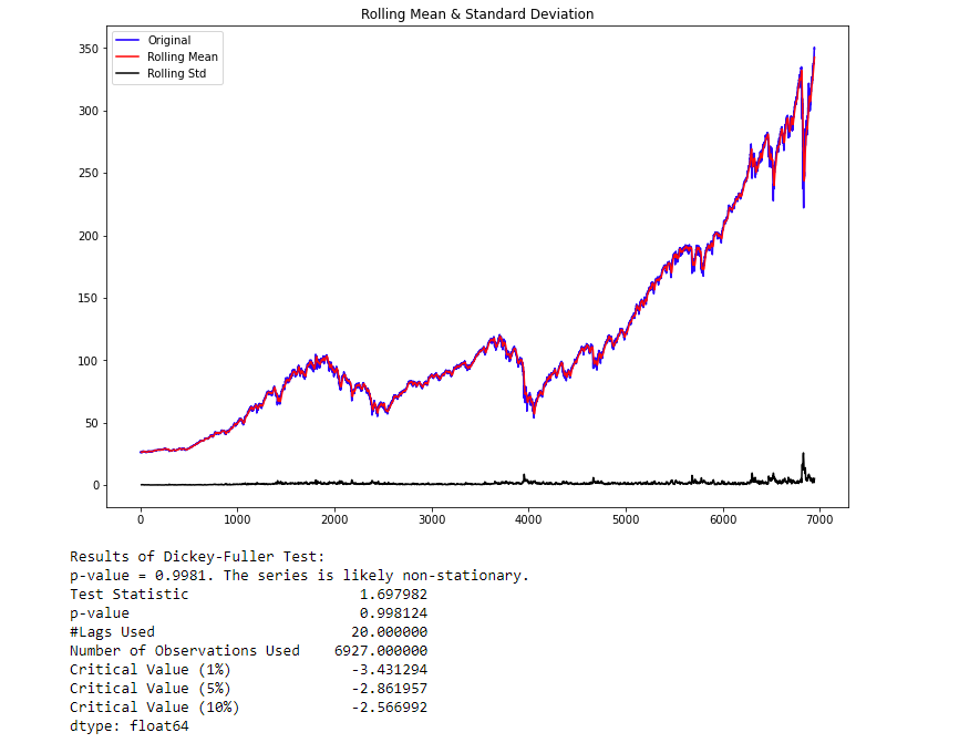

The p-value obtained is greater than the significance level of 0.05, and the ADF test statistic is greater than any of the critical values. There is no reason to reject the null hypothesis. So, the time series is non-stationary

獲得的p值大于0.05的顯著性水平，并且ADF測試統計量大于任何臨界值。 沒有理由拒絕零假設。 因此，時間序列是非平穩的

As you can see, this function gives you all the information necessary in case you forget. As we thought, the data is not stationary. To make the data stationary, we need to take the first-order difference of the data. Which is just a fancy way of saying subtract today’s close price from yesterday’s close price. As expected, Pandas has a handy function to do this for us.

如您所見，此功能可為您提供所有必要的信息，以防萬一您忘記了。 正如我們認為的那樣，數據不是固定的。 為了使數據穩定， 我們需要對數據進行一階差分。 這只是從昨天的收盤價中減去今天的收盤價的一種奇特的說法。 不出所料，熊貓為我們做到了這一點。

# Get the difference of each Adj Close point
spy_close_diff_1 = series.diff()# Drop the first row as it will have a null value in this column
spy_close_diff_1.dropna(inplace=True)

Now that we have attempted to make our data set stationary, let’s test it to be sure. Re-run test_stationarity(spy_close_diff_1).

現在，我們已經嘗試使數據集保持平穩，讓我們對其進行測試以確保確定。 重新運行test_stationarity(spy_close_diff_1)。

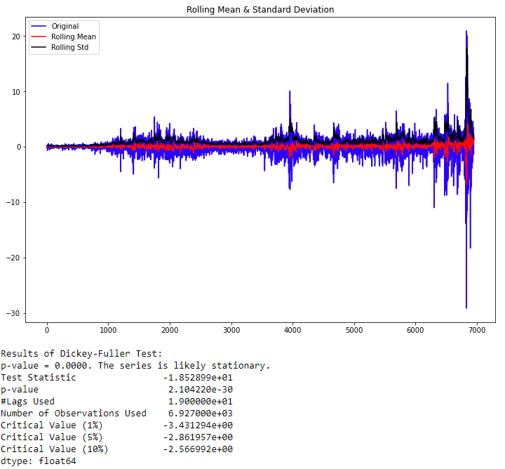
The p-value obtained is less than the significance level of 0.05, and the ADF statistic is lower than any of the critical values. We reject the null hypothesis. So, the time series is, in fact, stationary. Finally, our data is stationary, and we can continue. In some instances, you may have to do this more than once.

獲得的p值小于0.05的顯著性水平，并且ADF統計量低于任何臨界值。 我們拒絕原假設。 因此，時間序列實際上是固定的。 最后，我們的數據是固定的，我們可以繼續。 在某些情況下，您可能必須多次執行此操作。

步驟3：自相關和部分自相關 (Step 3: Autocorrelation and Partial Autocorrelation)

Autocorrelation is the correlation between points at time t (P?) and the point at(P???). Partial autocorrelation is the point at time t (P?) and the point (P???) where k is any number of lags. Partial autocorrelation ignores all of the data in between both points.

自相關是在時間t(P?)處的點與(p between)處的點之間的相關性。 局部自相關是時間t處的點(P?)和點(P number)，其中k是任意數量的滯后。 局部自相關會忽略兩點之間的所有數據。

In terms of a movie theater’s ticket sales, autocorrelation determines the relationship of today’s ticket sales and yesterday’s ticket sales. In comparison, partial autocorrelation defines the relationship of this Friday’s ticket sales and last Friday’s ticket sales.

就電影院的票務而言，自相關決定了今天的票務與昨天的票務之間的關系。 相比之下，部分自相關定義了此星期五的票務銷售與上周五的票務銷售之間的關系。

Here is a quick way to plot Autocorrelation and Partial Autocorrelation:

這是繪制自相關和部分自相關的快速方法：

from statsmodels.graphics.tsaplots import plot_acf,plot_pacfplot_acf(spy_close_diff_1)
plt.xlabel('Lags (Days)')
plt.show()# Break these into two separate cells
plot_pacf(spy_close_diff_1)
plt.xlabel('Lags (Days)')
plt.show()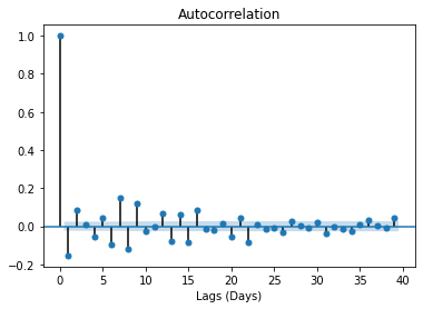

These plots look almost identical, but they’re not. Let’s start with the Autocorrelation plot. The important detail of these plots is the first lag. If the first lag is positive, we use an autoregressive (AR) model, and if the first lag is negative, we use a moving average (MA) plot. Since the first lag is negative, and the 2nd lag is positive, we will use the 1st lag as a moving average point.

這些圖看起來幾乎相同，但事實并非如此。 讓我們從自相關圖開始。 這些圖的重要細節是第一個滯后。 如果第一個滯后為正，則使用自回歸(AR)模型；如果第一個滯后為負，則使用移動平均(MA)圖。 由于第一個延遲為負，第二個延遲為正，因此我們將第一個延遲用作移動平均點。

For the PACF plot, since there is a substantial dropoff at lag one, which is negatively correlated, we will use an AR factor of 1 as well. If you have trouble determining how what lags are the best to use, feel free to experiment, and watch the AIC. The lower the AIC, the better.

對于PACF圖，由于滯后1處有一個很大的下降，它是負相關的，因此我們也將AR因子設為1。 如果您無法確定最佳使用滯后的方法，請隨時嘗試并觀看AIC。 AIC越低越好。

The ARIMA model takes three main inputs into the “order” argument. Those arguments are ‘p’ for the AR term, ‘d’ for the differencing term, ‘q’ for the MA term. We have determined the best model for our data is of order (1,1,1). Once again, feel free to change these numbers and print out the summary of the models to see which variation has the lowest AIC. The training time is relatively quick.

ARIMA模型將三個主要輸入納入“ order”參數。 這些參數對于AR項是“ p”，對于差分項是“ d”，對于MA項是“ q”。 我們確定最佳數據模型為(1,1,1)。 再一次，可以隨意更改這些數字并打印出模型摘要，以查看哪個版本的AIC最低。 訓練時間相對較快。

# Use this block to
from statsmodels.tsa.arima_model import ARIMA# fit model
spy_arima = ARIMA(x_train, order=(1,1,1))
spy_arima_fit = spy_arima.fit(disp=0)
print(spy_arima_fit.summary())

步驟4：預測 (Step 4: Forecasting)

Now that you have figured out which model has the best AIC score, I am using order = (1,1,1). Let’s use this model to make predictions on our test data set.. Now, I am sure there has to be a faster way of getting this done, but this is my approach. The run time on this cell may take some time. The run time is long because it moves across one data point at a time, refitting the model and creating a prediction for the next day. The last line of code is critical, as it is a magic command for Jupyter Notebook and will store the model predictions even if you restart your notebook’s kernel. This line will prevent you from having to rerun this cell in the future.

現在您已經確定了哪個模型的AIC得分最高，我在使用order =(1,1,1)。 讓我們使用此模型對測試數據集進行預測。現在，我確信必須有一種更快的方法來完成此操作，但這是我的方法。 在此單元格上的運行時間可能需要一些時間。 運行時間很長，因為它一次跨一個數據點移動，因此需要重新擬合模型并為第二天創建預測。 最后一行代碼很關鍵，因為它是Jupyter Notebook的神奇命令，即使重新啟動Notebook的內核，它也會存儲模型預測。 此行將防止您將來不得不重新運行此單元格。

# Create list of x train valuess
history = [x for x in x_train]# establish list for predictions
model_predictions = []# Count number of test data points
N_test_observations = len(x_test)# loop through every data point
for time_point in list(x_test.index):
    model = ARIMA(history, order=(1,1,1))
    model_fit = model.fit(disp=0)
    output = model_fit.forecast()
    yhat = output[0]
    model_predictions.append(yhat)
    true_test_value = x_test[time_point]
    history.append(true_test_value)
MAE_error = keras.metrics.mean_absolute_error(x_test, model_predictions).numpy()
print('Testing Mean Squared Error is {}'.format(MAE_error))%store model_predictions

Below is the code on how to reload the stored variable from the Jupyter magic command. It is also best practice to save and reload your model too.

以下是有關如何從Jupyter magic命令重新加載存儲的變量的代碼。 最好也保存和重新加載模型。

# %store model_predictions
%store -r model_predictions# Check to see if it reloaded
model_predictions[:5]# Load model
from statsmodels.tsa.arima.model import ARIMAResults
loaded = ARIMAResults.load('arima_111.pkl')

步驟5：可視化模型 (Step 5: Visualize your model)

It is always important to view your model’s outputs to understand how it handled specific situations in your data. You may find some peculiar behavior that could lead to further model improvements.

查看模型的輸出以了解其如何處理數據中的特定情況始終很重要。 您可能會發現一些特殊行為，這些行為可能導致進一步的模型改進。

from sklearn.metrics import mean_absolute_value
arima_mae = mean_absolute_error(x_test,model_predictions)
arima_mae

For this model, I used the mean absolute error as the loss function. I like this loss function for financial models because it is in units that are easy to imagine. The loss of the ARIMA(1,1,1) model was 2.788. This loss means the average difference between the actual value and the model’s predicted value was off by $2.79. Looking at the volatility over this period, I’d say $2.97 isn’t too bad with the crazy amount of volatility we have had over our testing period. Let’s plot the graph and see what it looks like upon further inspection.

對于此模型，我使用平均絕對誤差作為損失函數。 我喜歡金融模型的損失函數，因為它的單位很容易想象。 ARIMA(1,1,1)模型的損失為2.788。 這種損失意味著實際價值與模型預測價值之間的平均差額為$ 2.79。 觀察這段時期的波動性，我想說2.97美元對我們在測試期間所經歷的瘋狂波動性來說還算不錯。 讓我們繪制圖表，并查看進一步檢查的外觀。

plt.rcParams['figure.figsize'] = [10, 10]plt.plot(x_test.index[-100:], model_predictions[-100:], color='blue',label='Predicted Price')
plt.plot(x_test.index[-100:], x_test[-100:], color='red', label='Actual Price')
plt.title('SPY Prices Prediction')
plt.xlabel('Date')
plt.ylabel('Prices')
# plt.xticks(np.arange(881,1259,50), df.Date[881:1259:50])
plt.legend()
plt.figure(figsize=(10,6))
plt.show()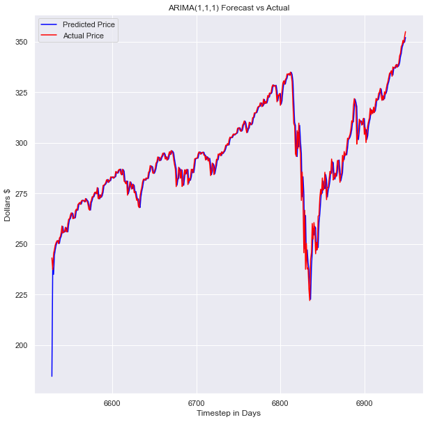

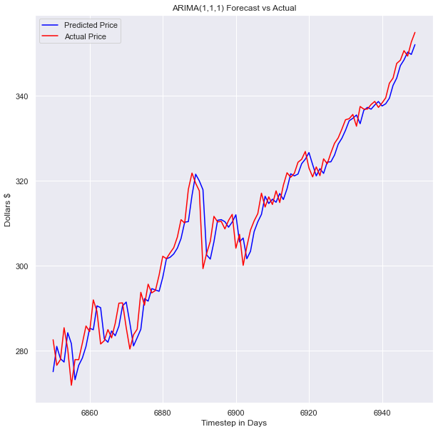
The model looks pretty good! Looking at the full test data set, you can’t see any space between our prediction and the actual values. This model performs well even when put up against more complex deep learning models. This model outperformed many of the deep learning models I built and trained on the same data sets.

模型看起來不錯！ 查看完整的測試數據集，您看不到我們的預測和實際值之間的任何空格。 即使遇到更復雜的深度學習模型，該模型也能很好地執行。 該模型優于我在同一數據集上構建和訓練的許多深度學習模型。

結論 (Conclusion)

Thank you for making it this far and reading my blog! I hope you enjoyed it and learned something from it. There is still a lot of work to be done to put this model before implementing this model into a trading system.

感謝您到目前為止所做的并閱讀我的博客！ 希望您喜歡它并從中學到一些東西。 在將此模型實現到交易系統之前，仍有很多工作要做。

Typical trading systems are a conglomeration of multiple models and data sources that output trading signals. It is crucial to understand how you want to use your model to generate trading signals, and then thoroughly backtest your model accounting for all trading costs. Only then should you try to implement your system on a paper trading account and see how it does.

典型的交易系統是輸出交易信號的多種模型和數據源的集合。 了解您要如何使用模型來生成交易信號，然后對所有交易成本進行全面回溯測試，這一點至關重要。 只有這樣，您才應該嘗試在紙幣交易帳戶上實施您的系統并查看其工作方式。

I have not yet gotten to those next stages, but when I do, I will be sure to share my findings!

我還沒有進入下一個階段，但是當我這樣做時，我一定會分享我的發現！

LinkedIn:

領英

www.linkedin.com/in/blakesamaha

www.linkedin.com/in/blakesamaha

Personal Website:

個人網站：

aggressiontothemean.com

aggressiontothemean.com

Twitter:

推特：

@Mean_Agression

@Mean_Agression