繪制大流行時期社區的風險群圖：以布宜諾斯艾利斯為例 (Map Risk Clusters of Neighbourhoods in the time of Pandemic: a case of Buenos Aires)

介紹 (Introduction)

Every year is unique and particular. But, 2020 brought the world the special planetary pandemic challenge of COVID-19. It spread and penetrated rapidly into different parts of the globe. And, the autonomous city of Buenos Aires (CABA: Ciudad Autonoma de Buenos Aires) is not an exception.

每年都是獨一無二的。 但是，2020年給世界帶來了COVID-19的特殊行星大流行挑戰。 它Swift傳播并滲透到全球各地。 而且，布宜諾斯艾利斯自治市(CABA：布宜諾斯艾利斯自治城市)也不例外。

In this particular setting, in order to craft the settings for my capstone project, I contemplated a hypothetical corporate client in the food industry (catering business) from abroad (The Client), that is planning to relocate their representative family to the city of Buenos Aires (CABA) for their future entry into Argentina once the pandemic-related restrictions are lifted. Since this would be its very first entry to Buenos Aires, the city is still an unknown territory for the Client.

在這個特殊的環境中，為了完善我的頂峰項目的環境，我考慮了一個來自國外(客戶)食品行業(餐飲業務)的假設企業客戶，該公司計劃將其代表家庭搬到布宜諾斯艾利斯市一旦取消與大流行有關的限制，Aires(CABA)便會在未來進入阿根廷。 由于這將是它第一次進入布宜諾斯艾利斯，因此該城市對于客戶來說仍然是一個未知的領域。

Very concerned with the two risks — the general security risk (crime) and the pandemic risk (COVID-19) — the Client wants to exclude high risk neighbourhoods in the selection of the location for the plan. In addition, the Client wants to capture the characteristics of neighbourhoods based on popular commercial venue categories such as restaurants, shops, and sports facilities. In this context, the Client hired me as an independent data analyst to conduct a preliminary research for its future plan.

客戶非常關注這兩種風險-一般安全風險(犯罪)和大流行風險(COVID-19)-客戶希望在選擇計劃的地點時排除高風險社區。 此外，客戶希望根據受歡迎的商業場所類別(例如餐廳，商店和體育設施)來捕捉社區的特征。 在這種情況下，客戶聘請我擔任獨立數據分析師，以對其未來計劃進行初步研究。

The Client stressed that this is the first-round preliminary analysis for a further extended study for business expansion. And based on the finding from this preliminary analysis, the Client wants to explore the scope of the future analysis. Simply put, the Client wants to conduct the preliminary analysis within a short period of time under a small budget to taste the flavour of the subject.

客戶強調，這是為進一步擴展業務擴展研究而進行的第一輪初步分析。 并且，基于此初步分析的結果，客戶希望探索未來分析的范圍。 簡而言之，客戶希望在短時間內以少量預算進行初步分析，以品嘗主題的味道。

The Client sets the following three objectives for this preliminary assignment.

客戶為此初步任務設定以下三個目標。

1. Identify outlier high risk neighbourhoods (the Outlier Neighbourhood/Cluster) in terms of these two risks — the general security risk (crime) and the pandemic risk (COVID-19).
   從這兩個風險(一般安全風險(犯罪)和大流行風險(COVID-19))中識別異常高風險社區(異常社區/集群)。
2. Segment non-outlier neighbourhoods into several clusters (the Non-Outlier Clusters) and rank them based on a single quantitative risk metric (a compound risk metric of the general security risk and the pandemic risk).
   將非離群的鄰域劃分為多個群集(非離群的群集)，并基于單個定量風險度量(一般安全風險和大流行風險的復合風險度量)對它們進行排名。
3. Use Foursquare API to characterize the Non-Outlier Neighbourhoods regarding popular venues. And if possible, segment Non-Outlier Neighbourhoods according to Foursquare venue profiles.
   使用Foursquare API來描述有關受歡迎場所的非離群社區。 并且，如果可能，請根據Foursquare場地配置文件對非離群區域進行細分。

The autonomous city of Buenos Aires (CABA) is a densely populated city: the total population of approximately 3 million in the area of 203 km2. And each neighbourhood has its own distinct size of area and population. The city is divided into 48 administrative division, aka ‘barrios’, to which I will refer simply as ‘neighbourhoods’ in this report.

布宜諾斯艾利斯自治市(CABA)是一個人口稠密的城市：總人口約300萬，面積203平方公里。 每個鄰域都有其自己獨特的面積和人口規模。 該市分為48個行政區，又名“ barrios”，在本報告中，我將其簡稱為“社區”。

The Client expressed their concern about the effect of the variability of population density among neighbourhoods. These two risks of the Client’s concern — the general security risk (crime) and the pandemic risk (COVID-19) — are likely affected by the population density profiles. Especially, the fact that ‘social distancing’ is a key to the prevention of COVID-19 suggests that population density is a significant attribute for the pandemic risk. In other words, the higher the population density, the higher the infection rate. The similar can be true for the general security risk. Obviously, this preconception needs to be assessed based on the actual data in the course of the project. This needs to be kept in mind for the analysis. Nevertheless, the Client ask me to scale risk metrics by ‘population density’ for the first round of the project.

客戶對鄰里人口密度變化的影響表示關注。 客戶關注的這兩個風險(一般安全風險(犯罪)和大流行風險(COVID-19))可能會受到人口密度狀況的影響。 特別是，“社會隔離”是預防COVID-19的關鍵這一事實表明，人口密度是大流行風險的重要屬性。 換句話說，人口密度越高，感染率越高。 對于一般的安全風險也是如此。 顯然，需要根據項目過程中的實際數據來評估這種先入之見。 分析時必須牢記這一點。 但是，客戶要求我在項目的第一輪中按“人口密度”來衡量風險指標。

Overall, the Client demonstrated high enthusiasm about Machine Learning and requested me to use machine learning models to achieve all these three objectives aforementioned.

總體而言，客戶表現出了對機器學習的高度熱情，并要求我使用機器學習模型來實現上述所有三個目標。

That is the background (business problem) scenario for this capstone project. On one hand, the scenario setting is totally hypothetical. On the other hand, the project handles real data.

這是此頂點項目的背景(業務問題)方案。 一方面，方案設置完全是假設的。 另一方面，項目處理實際數據。

Cut a long story short, for these three objectives presented above, I performed three different clustering machine-learning models. And I got three different lessons out of them. All of them are valuable. And in Discussion section of this article I will stress these different implications from the perspective of Data Science project management.

簡而言之，對于上述三個目標，我執行了三種不同的集群機器學習模型。 我從中學到了三堂課。 所有這些都是有價值的。 在本文的“ 討論”部分，我將從數據科學項目管理的角度強調這些不同的含義。

For now, I will invite you to walk through the process of the analysis.

現在，我將邀請您逐步進行分析。

The code of the project could be viewed in the following link of my GitHub repository:

可以在我的GitHub存儲庫的以下鏈接中查看項目的代碼：

· Code: https://github.com/Hyper-Phronesis/Capstone-1/blob/master/Capstone%20Three%20Different%20Lessons%20from%20Three%20Different%20Clusterings.ipynb

·代碼： https ： //github.com/Hyper-Phronesis/Capstone-1/blob/master/Capstone%20Three%20Different%20Lessons%20from%20Three%20Different%20Clusterings.ipynb

Now, let’s start.

現在，讓我們開始。

業務理解與分析方法 (Business Understanding and Analytical Approach)

At the beginning of a Data Science project, we need to clarify the following two basic questions

在數據科學項目開始時，我們需要澄清以下兩個基本問題

1. what needs to be solved. (Business Understanding)
   需要解決的問題。 (業務理解)
2. what kind of approach we need to make in order to achieve the objective. (Analytical Approach)
   為了達到目標，我們需要采取哪種方法。 (分析方法)

For the case of this project, the Client already has specified both. What the Client wants are risk profiling, venue profiling, and clustering of neighbourhoods. These are all about analysis of the status quo, in other words, descriptive analysis; or potentially, it might involve diagnostic (what happened or what are happening). In other words, the Client is not asking for a forecast (predictive analysis) or how to solve the problem (prescriptive analysis) — at least at this preliminary stage. These navigate the overall direction of our analysis.

對于此項目，客戶端已經指定了兩者。 客戶需要的是風險剖析，場所剖析和社區聚類。 這些都是關于現狀的分析，換句話說就是描述性分析。 或可能涉及診斷(發生了什么或正在發生什么)。 換句話說，至少在這個初步階段，客戶并沒有要求進行預測(預測分析)或如何解決問題(描述性分析)。 這些將指導我們分析的總體方向。

Now, all clear. Let’s mover to the next. Now, we start talking about data.

現在，一切都清楚了。 讓我們前進到下一個。 現在，我們開始討論數據。

A.數據部分 (A. Data Section)

A1。 資料需求： (A1. Data Requirements:)

By an analogy to cooking, Data Requirements is like a recipe, what ingredients we would need for cooking the dish: thus, what kind of data we would need for the analysis. The three objectives set by the Client determine the data requirements as follow:

類似于烹飪，“數據需求”就像一個食譜，說明我們烹飪菜肴所需的食材：因此，我們需要哪種數據進行分析。 客戶設定的三個目標確定數據要求如下：

(1) Basic information about the neighbourhoods in Buenos Aires.

(1)關于布宜諾斯艾利斯居民區的基本信息。

• The area and the population for each neighbourhood
  每個社區的面積和人口
• The geographical coordinates to determine the administrative border of each neighbourhood (for map visualization)
  確定每個鄰域的行政邊界的地理坐標(用于地圖可視化)

(2) Risk statistics:

(2)風險統計：

For the first and the second objectives, I would need to gather the following historical statistics to construct a compound risk metric to profile neighbourhoods from the perspectives of both the general insecurity risk (crime) and the pandemic risk (COVID-19).

對于第一個和第二個目標，我將需要收集以下歷史統計數據，以從一般不安全風險(犯罪)和大流行風險(COVID-19)的角度構建復合風險度量標準，以對街區進行概要分析。

• general security risk statistics (crime incidences) by neighbourhoods
  社區的一般安全風險統計(犯罪發生率)
• pandemic risk statistics (COVID-19 confirmed cases) by neighbourhoods
  社區的大流行風險統計(COVID-19確診病例)

(3) Foursquare Data:

(3)Foursquare數據：

For the third objective, the Client requires me to specifically use Foursquare API in order to characterise each Non-Outlier Neighbourhood.

對于第三個目標，客戶要求我專門使用Foursquare API來表征每個非離群社區。

A2。 數據源 (A2. Data Sources)

Based on the data requirements, I explored the publicly available data. Then, I encountered the following relevant sources.

根據數據需求，我探索了公開可用的數據。 然后，我遇到了以下相關資源。

(1) Basic info of the neighbourhoods of CABA:

(1)CABA社區的基本信息：

• the area and the population of all the relevant neighbourhoods from Wikipedia: https://en.wikipedia.org/wiki/Neighbourhoods_of_Buenos_Aires

  維基百科上所有相關社區的面積和人口： https ： //en.wikipedia.org/wiki/Neighbourhoods_of_Buenos_Aires

• The city government of Buenos Aires provides a GeoJson file that contains the geographical coordinates which defines the administrative boundary of Barrios (the neighbourhoods) of Buenos Aires. https://data.buenosaires.gob.ar/dataset/barrios/archivo/1c3d185b-fdc9-474b-b41b-9bd960a3806e

  布宜諾斯艾利斯市政府提供了一個GeoJson文件，其中包含地理坐標，該地理坐標定義了布宜諾斯艾利斯Barrios(社區)的行政邊界。 https://data.buenosaires.gob.ar/dataset/barrios/archivo/1c3d185b-fdc9-474b-b41b-9bd960a3806e

(2) Historical risk statistics.

(2)歷史風險統計。

• Crime Statistics: A csv file which is compiled and uploaded by Rama in his GitHub depository: https://github.com/ramadis/delitos-caba/releases/download/3.0/delitos.csv

  犯罪統計數據：一個由Rama在其GitHub存儲庫中編譯并上傳的csv文件： https ： //github.com/ramadis/delitos-caba/releases/download/3.0/delitos.csv

• COVID-19 Statistics: the city government’s website provides the COVID-19 statistics by neighbourhood: https://cdn.buenosaires.gob.ar/datosabiertos/datasets/salud/casos-covid-19/casos_covid19.xlsx

  COVID-19統計信息：市政府的網站按鄰居提供COVID-19統計信息： https ://cdn.buenosaires.gob.ar/datosabiertos/datasets/salud/casos-covid-19/casos_covid19.xlsx

(3) Foursquare Data for Popular Venues by Neighbourhood:

(3)各地區熱門場所的Foursquare數據：

As per the Client’s requirement, I would specifically use Foursquare API in order to characterise each Non-Outlier Neighbourhood.

根據客戶的要求，我將專門使用Foursquare API來表征每個非離群社區。

A3。 數據采集 (A3. Data Collection)

What follow now are data collection, data understanding, and data preparation. These parts altogether usually occupy a majority of time for the project, e.g. in a range of 60–70%.

現在，接下來是數據收集，數據理解和數據準備。 這些部分通常總共占項目的大部分時間，例如占60-70％。

For this article, I would compress the description of these time-consuming parts, by only outlining highlights.

對于本文，我將僅概述重點內容來壓縮這些耗時部分的描述。

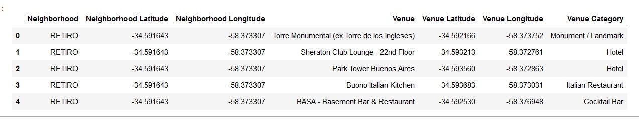
After downloading all the relevant data from the data sources above, I have made data reconciliation — cleaning data and transforming it in a coherent format. Thereafter, I consolidated all the relevant data into two datasets: “Risk Profile of Neighbourhoods” dataset and “Foursquare Venue Profile” dataset. The first 5rows of each dataset are presented below to illustrate their components.

從上面的數據源下載了所有相關數據之后，我進行了數據對帳-清理數據并將其轉換為一致的格式。 之后，我將所有相關數據合并為兩個數據集：“街區風險概況”數據集和“四方場地概況”數據集。 下面介紹了每個數據集的前5行，以說明它們的組成。

The first 5 rows of “Risk Profile of Neighbourhoods”:

“鄰里風險概況”的前5行：

The first 5 rows of “Foursquare Venue Profile”:

“四方場地簡介”的前5行：

Here is an outline of data limitation below.

以下是數據限制的概述。

(1) Crime Statistics: “Crime Severity Score”

(一)犯罪統計：“犯罪等級”

The compiled crime data covers only the period between Jan 1, 2016 and Dec 31, 2018. For the purpose of the project, I would make an assumption that the data during the available period would be good enough to serve a representative proxy for the risk characteristic of each neighbourhood.

匯總的犯罪數據僅涵蓋2016年1月1日至2018年12月31日期間。就本項目而言，我假設可用期間的數據足以為風險提供代表性代表每個社區的特征。

The original crime statistics had 7 crime categories. They were weighted according to the severity of crime category and transformed to generate one single metric “Crime Severity Score”.

原始犯罪統計數據有7種犯罪類別。 根據犯罪類別的嚴重程度對它們進行加權，然后轉換為一個度量“犯罪嚴重度評分”。

(2) COVID-19 Statistics: “COVID-19 Confirmed Cases”

(2)COVID-19統計：“ COVID-19確診病例”

In order to measure the pandemic risk, I simply extracted the cumulative confirmed cases of COVID-19 for each neighbourhood. I did not net out the recovered cases from the data. Thus, the COVID-19 statistics in this analysis is a gross figure. My assumption here is that the gross data will proxy the empirical risk profile of COVID-19 infection.

為了衡量大流行的風險，我只提取了每個社區累積的確診的COVID-19病例。 我沒有從數據中扣除恢復的案件。 因此，此分析中的COVID-19統計數據為毛值。 我在這里的假設是，總數據將替代COVID-19感染的經驗風險概況。

(3) Foursquare Data:

(3)Foursquare數據：

Foursquare API allows the user to explore venues within a user specified radius from one single location point. In other words, the user needs to specify the following parameters:

Foursquare API允許用戶從一個單一位置點探索用戶指定半徑內的場地。 換句話說，用戶需要指定以下參數：

• The geographical coordinates of one single starting point
  一個單一起點的地理坐標
• ‘radius’: The radius to set the geographical scope of the query.
  'radius'：設置查詢地理范圍的半徑。

This imposes a critical constraint in exploring venues within a neighbourhood from corner to corner. Since there is no uniformity in the area size among neighbourhoods, a compromise would be inevitable, while we want to capture the venue profile of a neighbourhood from corner to corner within its geographical border. Thus, the dataset that I would analyse for Foursquare venue analysis would be a geographically restrained sample set. I will use geopy’s Nominatim to obtain the representative single location point for each Neighbourhood.

這在探索社區內各個角落的場所時施加了嚴格的約束。 由于各社區之間的面積大小并不一致，因此在我們希望捕獲某個社區在其地理邊界內從一個角落到另一個角落的場地概況時，將不可避免地要做出折衷。 因此，我將對Foursquare場所分析進行分析的數據集將是一個受地理約束的樣本集。 我將使用geopy的Nominatim為每個街區獲得代表性的單個位置點。

A4。 數據理解 (A4. Data Understanding)

By now, the required data has been collected and reconciled. By an analogy to cooking, I have already cleaned and chopped the required ingredients according to the cook book. Now, I need to check the characteristics of the prepared ingredients: if they are representative of what we expected according to the cook book or othewise. Analogously, in this step of ‘data understanding’, I need to get an insight about the given data.

到現在為止，所需的數據已被收集和核對。 打個比方，我已經按照烹飪書清洗并切碎了所需的食材。 現在，我需要檢查準備好的食材的特性：它們是否代表我們根據烹飪書或其他所期望的內容。 類似地，在“數據理解”這一步驟中，我需要對給定數據有一個見解。

Repeatedly, I consolidated all the relevant data into two datasets: “Risk Profile of Neighbourhoods” dataset and “Foursquare Venue Profile” dataset. Let me analyse one by one.

我反復地將所有相關數據合并為兩個數據集：“街區風險概況”數據集和“四方場地概況”數據集。 讓我一一分析。

(1) “Risk Profile of Neighbourhoods” dataset:

(1)“鄰里風險概況”數據集：

For data understanding, there are several basic tools that helps us shape insights about the data distribution. And I performed the following three basic visualizations and generated one basic descriptive statistics:

為了了解數據，有幾種基本工具可幫助我們形成有關數據分布的見解。 我執行了以下三個基本可視化，并生成了一個基本的描述統計數據：

a) Scatter Matrix:

a)散布矩陣：

The scatter matrix below displays two types of distribution:

下面的分散矩陣顯示兩種分布類型：

• the individual distribution of each feature variable on the diagonal cells;
  每個特征變量在對角線上的單獨分布；
• the pair-wise distribution of data points for two feature variables.
  兩個特征變量的數據點的成對分布。

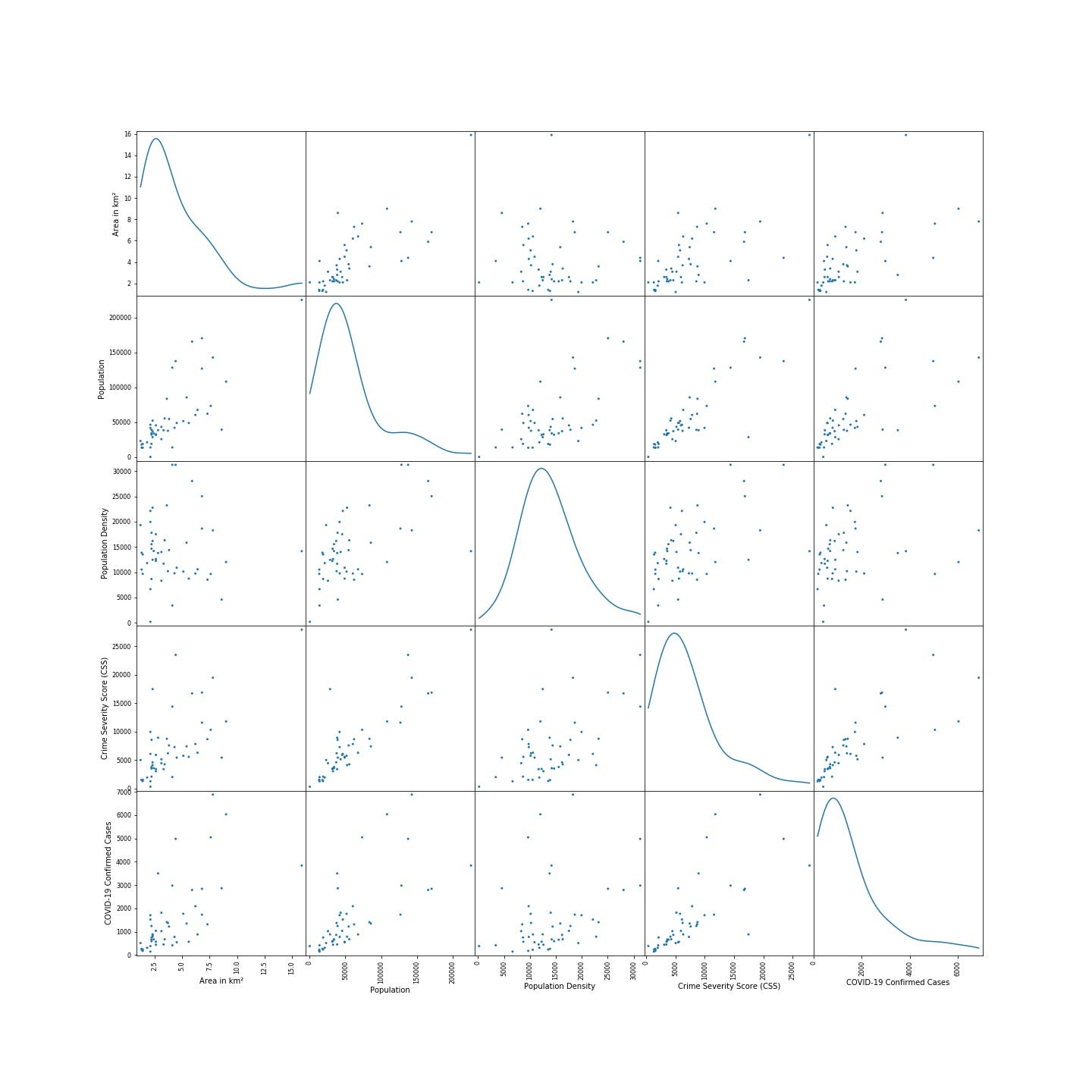
Here are some insights that I can derived from the scatter plot:

以下是我可以從散點圖中得出的一些見解：

• On the diagonal cells of the scatter matrix, all the data except ‘population density’ demonstrate highly skewed individual distributions, suggesting the presence of outliers.
  在散點圖矩陣的對角線上，除“人口密度”外，所有數據均顯示出高度偏斜的個體分布，表明存在異常值。
• In the off-diagonal cells, the most of the pair-wise plots suggest positive correlations in one way or another: except ‘population density’ with the area size and ‘COVID-19 Confirmed Cases’.
  在非對角線細胞中，大多數成對圖以一種或另一種方式表明正相關：除了“人口密度”與面積大小和“ COVID-19確診病例”。

b) Correlation Matrix:

b)相關矩陣：

In order to quantitatively capture the second insight above in one single table, I plotted the correlation matrix below.

為了在一個表格中定量地獲得上述第二個見解，我在下面繪制了相關矩陣。

Overall, “population density” stands out in the sense that it demonstrates relatively lower correlation with these two risk-metrics. On the other hand, population demonstrates the highest correlation with these two risk-metrics. This would raise a question: which feature — ‘area’, ‘population’ or ‘population density’ — would be the best to scale these two risk-metrics, ‘Crime Severity Score (CSS)’ and ‘COVID-19 Confirmed Cases’? This question needs to be reserved for a suggestion for the second round of this project.

總體而言，“人口密度”在與這兩個風險指標的相關性相對較低的意義上突出。 另一方面，人口與這兩個風險指標的相關性最高。 這就提出了一個問題：“面積”，“人口”或“人口密度”哪個特征將是最好的衡量這兩個風險指標的指標，“犯罪嚴重度評分(CSS)”和“ COVID-19確診病例” ？ 這個問題需要保留，以便對該項目第二輪提出建議。

Nevertheless, for this first round, as per the Client’s request to scale the risk metrics by population density, I scale these two-risk metrics with population density, by simply dividing the two risk-metrics by population density. As result, we have ‘CSS Index’ and ‘COVID-19 Index’.

不過，在第一輪中，根據客戶要求按人口密度縮放風險指標的要求，我將這兩個風險度量值按人口密度進行了縮放，只需將兩個風險指標除以人口密度即可。 結果，我們有了“ CSS索引”和“ COVID-19索引”。

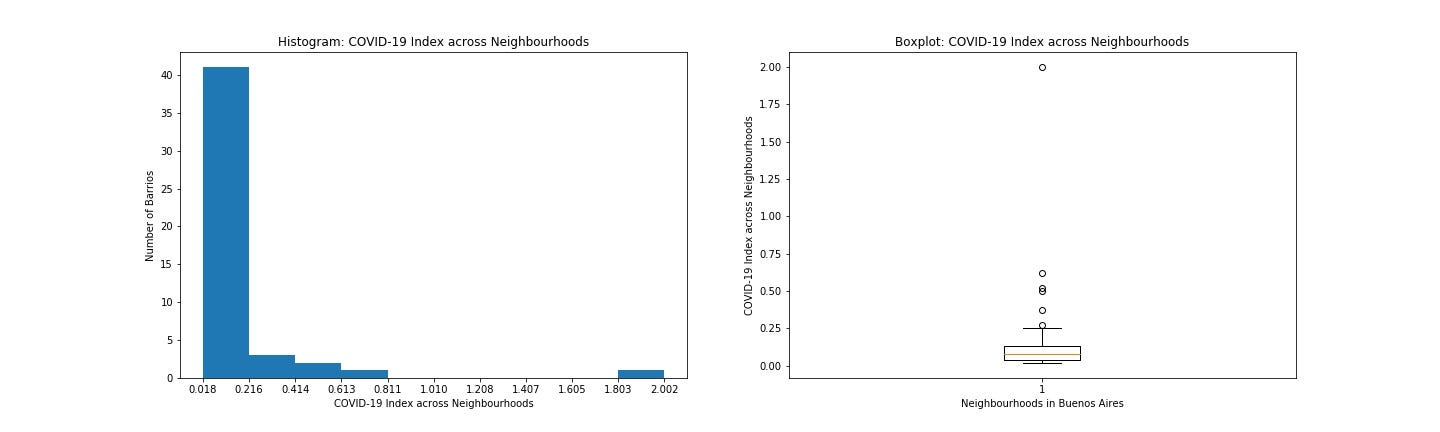
In order to study individual distributions for these newly created indices, I made the following two basic types of visualizations. Here are two pairs of histogram and boxplot, the first pair for ‘CSS Index’ and the second pair for ‘COVID-19 Index’.

為了研究這些新創建的索引的個體分布，我進行了以下兩種基本類型的可視化處理。 這是兩對直方圖和箱線圖，第一對為“ CSS索引”，第二對為“ COVID-19索引”。

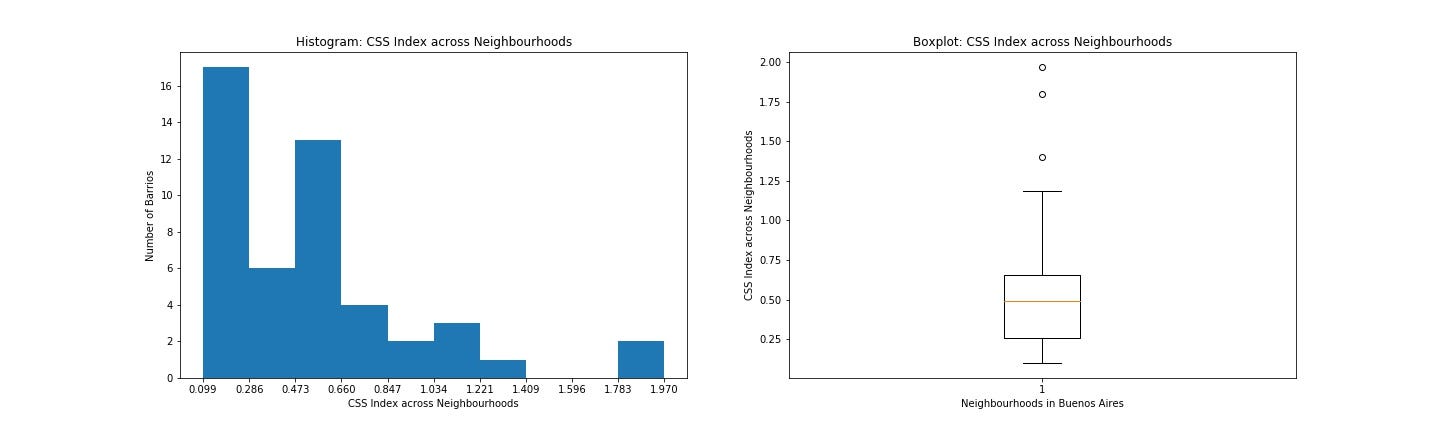
c) Histogram:

c)直方圖：

A histogram is useful to capture the shape of the distribution. It displays the distribution of data points across a pre-specified number of segmented ranges of the feature variable called bins. These two histograms (both on the left side) above visually warn the presence of outliers.

直方圖對于捕獲分布的形狀很有用。 它顯示在預先指定數量的稱為bins的特征變量的分段范圍內的數據點分布。 上方的這兩個直方圖(均在左側)警告存在異常值。

d) Boxplot:

d)箱線圖：

A boxplot displays the distribution of data according to descriptive statistics of percentiles: e.g. 25%, 50%, 75%. For our data, the boxplots above (on the right side) isolated outliers over their top whiskers. The tables below present more detailed info about these outliers from these two boxplots.

箱形圖根據百分位的描述性統計顯示數據分布：例如25％，50％，75％。 對于我們的數據，上方(右側)的箱線圖將其頂部晶須上的離群值隔離了。 下表列出了來自這兩個箱形圖的這些離群值的詳細信息。

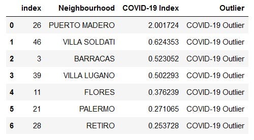
There are some overlapping outlier neighbourhoods between these two lists. Consolidating them, here is the list of 8 overall risk outliers.

這兩個列表之間存在一些重疊的離群鄰域。 合并它們，以下是8個總體風險異常值的列表。

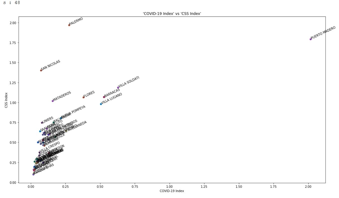
Now, let me plot the neighbourhoods on the two-dimensional risk space: ‘CSS Index’ and ‘COVID-19 Index’. The scatter plot below also helps us confirm these outliers visually.

現在，讓我在二維風險空間上繪制鄰域：“ CSS索引”和“ COVID-19索引”。 下面的散點圖還有助于我們從視覺上確認這些異常值。

These simple visualizations and descriptive statistics can be a very powerful tool and it helps us shape an insight about the data at the stage of Data Understanding. In a way, before clustering analysis, the boxplot and the scatter plot have already spotted outliers.

這些簡單的可視化和描述性統計信息可能是一個非常強大的工具，它可以幫助我們在“數據理解”階段塑造有關數據的見解。 在某種程度上，在進行聚類分析之前，箱線圖和散點圖已經發現了異常值。

(2) “Foursquare Venue Profile” dataset:

(2)“四方場地概況”數據集：

Here is the summary of the Foursquare response to my query. In order to obtain an insight about the distribution of the response across different neighbourhoods, the histogram and the boxplot are presented below.

這是對我的查詢的Foursquare響應的摘要。 為了深入了解不同社區的響應分布，下面介紹了直方圖和箱形圖。

The histogram might suggest that there might be some issues in the coherency of data quality and availability across different neighbourhoods. If that is the case, this might affect the quality of the result of clustering machine learning.

直方圖可能表明不同社區之間數據質量和可用性的一致性可能存在一些問題。 如果真是這樣，這可能會影響群集機器學習結果的質量。

Just in case, I would like to see if there is any relationship between the Foursquare’s response and the three basic profiles of neighbourhoods. I generated the correlation matrix and the scatter matrix.

為了以防萬一，我想看看Foursquare的回答和三個基本街區之間是否有任何關系。 我生成了相關矩陣和散射矩陣。

Here is an intuitive outcome. Venue response has the highest correlation with population density and the least correlation with the area size of neighbourhoods. In other words, the scatter matrix and the correlation matrix suggest that the higher the population density, the more venue information Foursquare has for neighbourhoods. It appeals to our common sense in a way: densely populated busy neighbourhoods have more venues.

這是一個直觀的結果。 場地響應與人口密度的相關性最高，而與社區面積的相關性則最小。 換句話說，散布矩陣和相關矩陣表明，人口密度越高，Foursquare提供給附近社區的場所信息越多。 它在某種程度上吸引了我們的常識：人口稠密的繁忙社區擁有更多場地。

For the rest of my work in data collection, data understanding, and data preparation, I would leave it up to the reader to see more detail in my code in the link above.

在數據收集，數據理解和數據準備的其余工作中，我將留給讀者以查看上面鏈接中的代碼中的更多細節。

方法論與分析 (B. Methodology & Analysis)

Now, the data is prepared for analysis. So, I can move on to analysis

現在，數據已準備好進行分析。 所以，我可以繼續分析

The three objectives set by the Client at the outset and the data availability that I confirmed determine the scope of methodology. Cut a long story short, I run three clustering machine learning models for three different objectives and I got three very different lessons from them.

客戶一開始設定的三個目標以及我確認的數據可用性決定了方法的范圍。 簡而言之，我針對三個不同的目標運行了三個集群機器學習模型，從中我得到了三個非常不同的教訓。

Before proceeding further, let me review the three objectives here.

在繼續進行之前，讓我在這里回顧三個目標。

1. Identify outlier high risk neighbourhoods (outlier neighbourhoods/clusters) in terms of these two risks — the general security risk (crime) and the pandemic risk (COVID-19).
   從這兩個風險(一般安全風險(犯罪)和大流行風險(COVID-19))中識別異常高風險社區(異常社區/集群)。
2. Segment non-outlier neighbours into several clusters (the non-outlier neighbourhoods/clusters) and rank them based on a single quantitative risk metric (a compound risk metric of the general security risk and the pandemic risk).
   將非離群的鄰居劃分為幾個集群(非離群的鄰居/集群)，并基于單個定量風險度量(一般安全風險和大流行風險的復合風險度量)對它們進行排名。
3. Use Foursquare API to characterize the Non-Outlier Neighbourhoods regarding popular venues. And if possible, segment Non-Outlier Neighbourhoods according to popular venue profiles.
   使用Foursquare API來描述有關受歡迎場所的非離群社區。 并且，如果可能的話，請根據受歡迎的場所概況細分非離群地區。

Now, there presents one common salient feature among these three objectives. We have no ‘a priori knowledge’ about the underlying cluster structure of any of the subjects: outlier neighbourhoods, non-outlier neighbourhoods, and popular venue profiles among non-outlier neighbourhoods. Simply put, unlike supervised machine learning models, we have no labelled data to train: we have no empirical data about the dependent variable. All these three objectives demand us to discover hidden labels, or unknown underlying cluster structures in the dataset.

現在，這三個目標之間呈現出一個共同的顯著特征。 我們沒有關于任何主題的基礎集群結構的“ 先驗知識”：離群社區，非離群社區以及非離群社區中的熱門場館概況。 簡而言之，與有監督的機器學習模型不同，我們沒有要訓練的標記數據：沒有因變量的經驗數據。 所有這三個目標都要求我們發現數據集中的隱藏標簽或未知的基礎簇結構。

This feature would naturally navigate us to the territory of unsupervised machine learning, and more specifically, ‘Clustering Machine Learning’ in our context.

此功能很自然地使我們導航到無監督機器學習的領域，更具體地講，在我們的上下文中是“集群機器學習”。

By its design — in the absence of the labelled data (empirical data for the dependent variable) — it would be difficult to automate the validation/evaluation process for an unsupervised machine learning, simply because there is no empirical label to compare the model outputs with. According to Dr. Andrew Ng, there seems no widely accepted consensus about clear cut methods to assess the goodness of fit for clustering machine learning models. This creates an ample room for human insight, such as domain/business expertise, to get involved in the validation/evaluation process.

通過其設計-在沒有標記數據(因變量的經驗數據)的情況下-很難自動化無監督機器學習的驗證/評估過程，這僅僅是因為沒有經驗標簽可以將模型輸出與。 據吳安德(Andrew Ng)博士說，似乎沒有一種明確的方法可以用來評估聚類機器學習模型的適用性 。 這為諸如域/業務專業知識之類的人類見識創造了足夠的空間，以參與驗證/評估過程。

In this context, for this project, I will put more emphasis on tuning the model a priori rather than pursuing the automation of the a posteriori validation/evaluation process.

在這種情況下，對于這個項目，我將更加強調先驗地調整模型，而不是追求后驗驗證/評估過程的自動化。

As one more important thing to mention, we need to normalize/standardize all the input data before passing them to machine learning models.

值得一提的是，我們需要在將所有輸入數據傳遞到機器學習模型之前對其進行標準化/標準化。

Now, I will discuss the methodologies for each objective one by one.

現在，我將逐個討論每個目標的方法。

B1。 針對目標1的DBSCAN集群： (B1. DBSCAN Clustering for Objective 1:)

The first objective is to identify ‘Outlier Neighbourhoods’.

第一個目標是確定“異常地區”。

Now, in the scatter plot below, all the neighbourhoods are plotted in the two-dimensional risk space: ‘CSS Index’ vs ‘COVID-19 Index’ space.

現在，在下面的散點圖中，所有鄰域都在二維風險空間中繪制：“ CSS索引”與“ COVID-19索引”空間。

In order to identify outliers out of these “two-dimensional spatial data points”, I chose DBSCAN Clustering model, or Density-based Spatial Clustering of Applications with Noise. As its name suggests, DBSCAN is a density-based clustering algorithm and deemed appropriate for examining spatial data. Especially, I am very interested in how the density-based clustering algorithm would process outliers which are expected to demonstrate extremely sparse density.

為了從這些“二維空間數據點”中識別離群值，我選擇了DBSCAN聚類模型 ，即基于噪聲的應用程序的基于密度的空間聚類 。 顧名思義，DBSCAN是基于密度的聚類算法，被認為適合檢查空間數據 。 尤其是，我對基于密度的聚類算法如何處理離群值異常稀疏的異常非常感興趣。

There are several hyperparameters for DBSCAN. And the one considered as the most crucial is ‘eps’. According to the Skit-learn.org website, ‘eps’ is:

DBSCAN有幾個超參數。 被認為是最關鍵的一個是“ eps ”。 根據Skit-learn.org網站，“ eps ”為：

“the maximum distance between two samples for one to be considered as in the neighborhood of the other. This is not a maximum bound on the distances of points within a cluster. This is the most important DBSCAN parameter to choose appropriately for your data set and distance function.” (https://scikit-learn.org/stable/modules/generated/sklearn.cluster.DBSCAN.html)

“一個樣本的兩個樣本之間的最大距離應視為另一個樣本的鄰域。 這不是群集中點的距離的最大界限。 這是 為您的數據集和距離函數適當選擇 的最重要的DBSCAN參數 。” ( https://scikit-learn.org/stable/modules/generated/sklearn.cluster.DBSCAN.html )

In order to tune ‘eps’, I will use KneeLocator of the python library kneed to identify the knee point (or elbow point).

為了調諧“EPS”，我將使用KneeLocator的Python庫用膝蓋 識別拐點 (或肘點)。

What is the knee point?

拐點是什么？

One way to interpret the knee point is that it is a point where the tuning results start converging within a certain acceptable range. Simply put, it is a point where further tuning enhancement would no longer yield a material incremental benefit. In other words, the knee point determines a cost-benefit boundary for model hyperparameter tuning enhancement.(Source: https://ieeexplore.ieee.org/document/5961514)

一種解釋拐點的方法是，在該點上，調整結果開始在某個可接受的范圍內收斂。 簡而言之，在這一點上進一步的調優將不再產生實質性的增量收益。 換句話說， 拐點確定了模型超參數調整增強的成本效益邊界 。(來源： https : //ieeexplore.ieee.org/document/5961514 )

In order to discover the knee point of the model hyperparameter, ‘eps’, for DBSCAN model, I passed the normalized/standardized data of these two risk indices — namely ‘Standardized CSS Index’ and ‘Standardized COVID-19 Index’ — into the KneeLocator.

為了發現模型超參數“ EPS” 的拐點 ，對于DBSCAN模型，我將這兩個風險指數(即“標準化CSS指數”和“標準化COVID-19指數”)的標準化/標準化數據傳遞給了KneeLocator 。

And here is the plot result:

這是繪圖結果：

The crossing point between the distance curve and the dotted straight vertical line identifies the knee point. Above the chart, KneeLocator also returned the one single value, 0.494, as the knee point. KneeLocator is telling me to choose this value as ‘eps’ to optimize the DBSCAN model. Accordingly, I plug it into DBSCAN. And here is the result.

距離曲線和垂直虛線之間的交點表示拐點。 在圖表上方， KneeLocator還返回了一個單一值0.494作為拐點 。 KneeLocator告訴我選擇此值作為'eps'以優化DBSCAN模型。 因此，我將其插入DBSCAN 。 這就是結果。

With this plot, I can confirm that DBSCAN distinguished the sparsely distributed outliers from others, yielding two clusters for them: the cluster -1 (light green) and the cluster 1 (orange). Below, I list up all the neighbourhoods of these two sparse clusters.

通過此圖，我可以確認DBSCAN可以將稀疏分布的異常值與其他異常值區分開，從而為它們生成兩個聚類：聚類-1(淺綠色)和聚類1(橙色)。 下面，我列出了這兩個稀疏群集的所有鄰域。

Furthermore, in order to assess if the result at the knee point is good or not, I run DBSCAN with other different values of ‘eps’. Here is the result:

此外，為了評估拐點處的結果是否良好，我使用其他不同的“ eps”值運行DBSCAN。 結果如下：

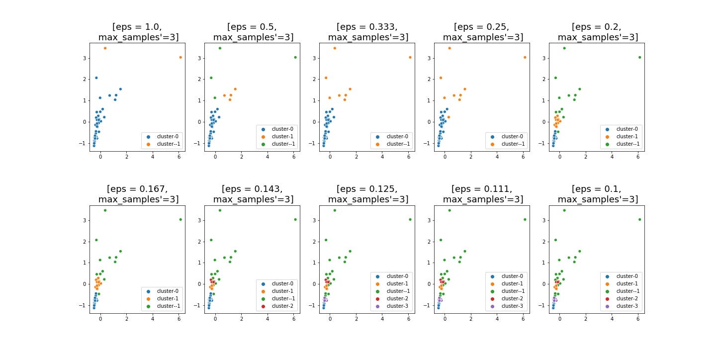
Compared with the result of the knee point ‘eps’, no alternative above would give us a better convincing result. Thus, I will not reject the knee point, the output of KneeLocator, as the value for the hyperparameter, ‘eps’.

與拐點 “ eps”的結果相比，上述任何選擇都不能給我們帶來更好的說服力。 因此，我不會拒絕拐點，即KneeLocator的輸出，作為超參數“ eps”的值。

When I look at the result of DBSCAN, I realise that this clustering result isolated into two clusters the same neighbourhoods as the outliers that the boxplot visualization identified during the Data Understanding stage.

當我查看DBSCAN的結果時，我意識到該聚類結果被隔離為兩個聚類，它們與盒形圖可視化在數據理解階段確定的離群值相同。

For your reminder, here is the result of the boxplot once again.

提醒您，這是箱線圖的結果。

The contents of these two results are identical (except for the order of the list). What does it tell us?

這兩個結果的內容是相同的(列表的順序除外)。 它告訴我們什么？

Now, the question worthwhile to ask would be: if we needed to perform a sophisticated and expensive model such as DBSCAN to identify outliers, when the simple boxplot can do that job.

現在，值得提出的問題是：當簡單的箱形圖可以完成此工作時，是否需要執行復雜且昂貴的模型(例如DBSCAN)來識別異常值。

In the perspective of cost-benefit management, the simple boxplot did the same job for the less cost — almost no cost. This might not be true when we have different data: especially, in a high-dimensional datapoints.

從成本效益管理的角度來看，簡單的箱線圖以較低的成本完成了相同的工作-幾乎沒有成本。 當我們擁有不同的數據時，尤其是在高維數據點中，情況可能并非如此。

At least, we should take this lesson in modesty so that we should not underestimate the power of simple methods like the boxplot visualisation.

至少，我們應該謹慎地學習本課，以免低估箱形圖可視化等簡單方法的功能。

B2。 第二個目標的層次聚類 (B2. Hierarchical Clustering for the second objective)

Now, the second objective can be broken down into the following core sub-objectives:

現在，第二個目標可以分解為以下核心子目標：

1. Segmentation of ‘Non-Outlier Neighbourhoods’.
   “非離群社區”的細分。
2. Construction of a single compound risk metric to measure both the general security risk and the pandemic risk.
   構建一個單一的復合風險度量以同時測量一般安全風險和大流行風險。
3. Measuring the risk profile at cluster level (not datapoints/neighbourhoods level).
   在群集級別(不是數據點/社區級別)上測量風險狀況。

a) Segmentation of ‘Non-Outlier Neighbourhoods’.

a) “非離群社區”的細分。

Given the result of the first objective, now I can remove “Outlier Neighbourhoods” from our dataset and focus only on “Non-Outlier Neighbourhoods” for further clustering segmentations.

有了第一個目標的結果，現在我可以從數據集中刪除“離群值鄰域”，而僅關注“非離群值鄰域”以進一步進行聚類分割。

This time, I choose Hierarchical Clustering model. Here are the reasons why I selected this particular model for the second objective:

這次，我選擇層次聚類模型。 這是我選擇此特定模型作為第二個目標的原因：

• I have no advance knowledge how many underlying clusters are expected in the dataset. Many clustering models, paradoxically, require the number of clusters as a hyperparameter input to tune the models a priori. But, Hierarchical Clustering doesn’t.

  我尚不了解在數據集中需要多少個基礎群集。 矛盾的是，許多聚類模型要求將聚類的數量作為超參數輸入來對模型進行先驗調整。 但是，分層聚類卻不是。

• In addition, Hierarchical Clustering algorithm can generate a dendrogram that illustrates a tree-like cluster structure based on the hierarchical structure of the pairwise spatial distance distribution. The ‘dendrogram’ appeals to our human intuition in discovering the underlying cluster structure.
  另外，分層聚類算法可以基于成對空間距離分布的分層結構生成樹狀圖，該樹狀圖說明樹狀聚類結構。 “樹狀圖”吸引了我們人類的直覺，從而發現了潛在的簇結構。

What is a dendrogram? Seeing is understanding! Maybe. Here you go:

什么是樹狀圖？ 眼見為諒！ 也許。 干得好：

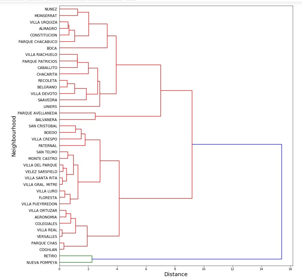
The dendrogram allows the user to study the hierarchical structure of distances among datapoints and the underlying layers of cluster hierarchy. The dendrogram analyses and displays the hierarchical structure of all the potential clusters automatically. The resulting dendrogram illustrates a tree-like cluster structure based on the pairwise distance distribution. In this way, the dendrogram allows the user to design how many clusters to be made for further analysis. We can visually confirm the hierarchy of the distances among data points and the layers of cluster structure in the dendrogram.

樹狀圖允許用戶研究數據點之間的距離的層次結構以及群集層次結構的基礎層。 樹狀圖自動分析并顯示所有潛在簇的層次結構。 生成的樹狀圖顯示了基于成對距離分布的樹狀群集結構。 這樣，樹狀圖使用戶可以設計要進行進一步分析的群集數。 我們可以從視覺上確認數據點之間的距離的層次結構以及樹狀圖中的簇結構層。

• From this dendrogram, I choose 4 (at the distance of 5 or 6 on the x-axis in the dendrogram) as the number of clusters to be shaped.
  從該樹狀圖中，我選擇4(在樹狀圖的x軸上距離5或6)作為要成形的簇的數量。
• Then, I run Hierarchical Cluster Model for the second time, this time with the specification of the number of the clusters, 4.
  然后，我第二次運行Hierarchical Cluster Model，這是在指定簇數為4的情況下進行的。

Accordingly, I got the 4 clusters of the neighbourhoods. The following two charts present the clustered neighbourhoods on the two risk-metrics space: one with neighbourhoods’ names and the other without.

因此，我得到了周圍的4個集群。 以下兩個圖表顯示了兩個風險度量空間上的聚類鄰域：一個帶有鄰域名稱，另一個沒有鄰域名稱。

In order to assign these clusters risk values. I will construct one single compound risk metric.

為了分配這些集群風險值。 我將構建一個單一的復合風險度量。

b) Construction of Compound Risk Metric

b)構建復合風險度量

I need to compress the two risk profiles of clusters (‘CSS’ and ‘COVID-19’) together into one single compound metric in order to achieve one of the Client’s requirement.

我需要將群集的兩個風險概況(“ CSS”和“ COVID-19”)壓縮到一個單一的復合指標中，以實現客戶的要求之一。

For this purpose, I formulated a compound risk metric as follows.

為此，我制定了如下的復合風險度量。

Compound Risk Metric =

復合風險指標=

[(Standardized CSS Index — Standardized Origin of CSS Index)2 +

[((標準化CSS索引-標準化CSS索引的來源)2+

(Standardized COVID-19 Index — Standardized Origin of COVID-19 Index)2 ]^0.5

(標準化的COVID-19索引-標準化的COVID-19索引來源)2] ^ 0.5

Although the formula might appear not straightforward, its basic intent is very simple: to measure the risk position of each neighbourhood from the risk-free point in the two-dimensional risk space.

盡管該公式可能看起來并不簡單，但是其基本意圖卻非常簡單：從二維風險空間中的無風險點測量每個鄰域的風險位置。

For the raw data, the risk-free point is at the origin of the two-risk-metrics space, which is (0,0): 0 represents no risk in the raw data. The formula above is measuring the risk position of a data point from the risk-free point after the standardization/normalization transformation. It is because in order to pass the data into the machine learning model, the data needs to be normalized/standardized. In that sense, the formula above measures the distance between the standardized data points and the standardized risk-free position.

對于原始數據，無風險點位于兩個風險度量空間的起點，即(0,0)：0表示原始數據中無風險。 上面的公式從標準化/規范化轉換后的無風險點開始測量數據點的風險位置。 這是因為為了將數據傳遞到機器學習模型中，需要對數據進行標準化/標準化。 從這個意義上講，上面的公式測量了標準化數據點和標準化無風險頭寸之間的距離。

Nothing else. That’s all and simple.

沒有其他的。 就是這么簡單。

b) Risk Profile of Cluster

b)集群風險簡介

Now, my ultimate purpose here is to quantify the risk profile at cluster level, not at data point/neighbourhood level.

現在，我的最終目的是在集群級別而不是數據點/社區級別量化風險狀況。

Each cluster has its own unique centre, aka “centroid”. Thus, in order to measure the risk profile of each cluster, I can refer to the centroid for each cluster. In this way, I can grade and rank all these clusters according to the compound risk metric of their centroids.

每個簇都有自己獨特的中心，又稱“ 質心 ”。 因此，為了衡量每個群集的風險狀況，我可以參考每個群集的質心。 這樣，我可以根據其質心的復合風險度量對所有這些聚類進行分級和排名。

Accordingly, I measure the compound risk metric of the centroids of all these 5 Non-Outlier Clusters and assign each of them a grade.

因此，我測量了所有這5個非異常值聚類的質心的復合風險度量，并為其分配了一個等級。

Here is the result.

這是結果。

The higher the grade, the riskier the cluster. I merged this result with the master dataset and assigned the cluster grade 5 to the 2 outlier clusters. Then, I mapped these cluster grades of all the neighbourhoods across CABA in the following Choropleth Map.

等級越高，集群的風險就越高。 我將此結果與主數據集合并，并將5級聚類分配給2個離群聚類。 然后，在下面的Choropleth映射中，我繪制了CABA中所有鄰域的這些聚類等級。

This map visually summarises the findings for these first two objectives. It allows the user to visually distinguish neighbourhood clusters across the autonomous city of Buenos Aires based on their cluster risk grade.

該地圖直觀地總結了前兩個目標的發現。 它使用戶能夠根據布宜諾斯艾利斯自治城市的聚類風險等級在視覺上區分其附近的聚類。

B1。 第三個目標的Foursquare分析 (B1. Foursquare Analysis for the third objective)

For the third objective, I used Foursquare data to carry out two analyses: Popular Venue Analysis; and Segmentation of Neighbourhoods based on Venue Composition.

對于第三個目標，我使用Foursquare數據進行了兩個分析：流行場地分析； 場地組成的鄰域細分。

a) Popular Venue Analysis:

a)流行場地分析：

I apply One Hot Encoding algorithm to transform the data structure of venue category for further data transformation.

我應用一種熱編碼算法來轉換會場類別的數據結構，以進行進一步的數據轉換。

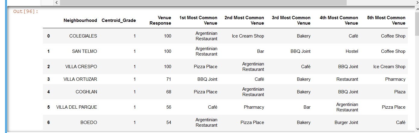
With Foursquare data, which has venue-base information, I will use Pandas’ “groupby” method to transform it to a neighbourhood-base data and summarise the top 5 popular venue categories for each of 40 ‘Non-Outlier Neighbourhoods’. The result is a very long list thus, I only display the first 7 lines.

借助具有場地基礎信息的Foursquare數據，我將使用Pandas的“ groupby”方法將其轉換為基于鄰域的數據，并總結40個“非離群鄰域”中每一個的前5個熱門場所類別。 結果是一個很長的列表，因此，我只顯示前7行。

b) Segmentation of Neighbourhoods based on Venue Profile

b)根據場地概況對鄰域進行細分

Next, I need to segment the Foursquare venue profile of each neighbourhood. For this purpose, I contemplate K-Means Clustering Machine Learning.

接下來，我需要細分每個社區的Foursquare場地概況。 為此，我打算使用K-Means集群機器學習。

For a successful K-Means clustering result, I need to determine one of its hyperparameters, n_clusters: the number of clusters to form, thus, the number of centroids to generate. (source: https://scikit-learn.org/stable/modules/generated/sklearn.cluster.KMeans.html)

為了獲得成功的K均值聚類結果，我需要確定其超參數之一n_clusters：要形成的簇數，因此要生成的質心數。 (來源： https : //scikit-learn.org/stable/modules/generated/sklearn.cluster.KMeans.html )

I will run two hyperparameter tuning methods — K-Means Elbow Method and Silhouette Score Analysis — to tune its most important hyperparameter, n_clusters. These tuning methods would give me an insight about how to cluster the data for a meaningful analysis. Based on the findings from these tuning methods, I would decide how to implement the K-Means Clustering machine learning model.

我將運行兩種超參數調整方法-K-Means彎頭方法和Silhouette Score分析-調整其最重要的超參數n_clusters。 這些調優方法將使我對如何對數據進行聚類進行有意義的分析有深刻的了解。 基于這些調整方法的發現，我將決定如何實施K-Means聚類機器學習模型。

‘K-Means Elbow Method’

“ K-均值肘法”

The spirit of ‘K-Means Elbow Method’ is the same as the knee point method that I explained earlier. Elbow locates a point where further tuning enhancement would no longer yield a material incremental benefit. In other words, Elbow determines a cost-benefit boundary for model hyperparameter tuning enhancement. Here is the result of K-Means Elbow Method:

“ K均值肘部彎曲法”的精神與我之前介紹的拐點法相同。 彎頭定位在一個點上，進一步的調音增強將不再產生實質性的增量收益。 換句話說， Elbow確定了模型超參數調整增強的成本效益邊界。 這是K-均值肘法的結果：

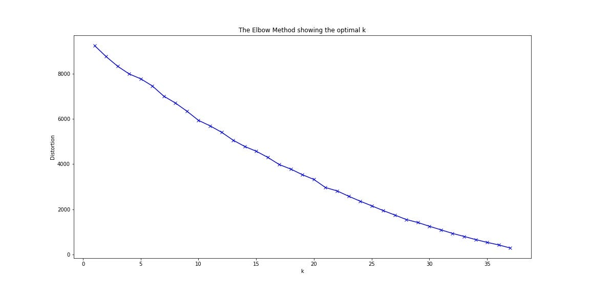
As the number of clusters increases, the response does not converge into any range; instead, it keeps dropping. There is no knee/elbow, the cost-benefit boundary, in the entire space. This suggests that there might be no meaningful cluster structure in the dataset. This is a disappointing result.

隨著簇數的增加，響應不會收斂到任何范圍。 相反，它一直在下降。 整個空間中沒有膝蓋/肘部，即成本效益邊界。 這表明數據集中可能沒有有意義的聚類結構。 這是令人失望的結果。

Silhouette Score Analysis

輪廓分數分析

https://scikit-learn.org/stable/auto_examples/cluster/plot_kmeans_silhouette_analysis.html

https://scikit-learn.org/stable/auto_examples/cluster/plot_kmeans_silhouette_analysis.html

Silhouette analysis can be used to study the separation distance between the resulting clusters. The silhouette plot displays a measure of how close each point in one cluster is to points in the neighbouring clusters and thus provides a way to assess parameters like number of clusters visually. This measure has a range of [-1, 1].

輪廓分析可用于研究所得簇之間的分離距離。 輪廓圖顯示了一個群集中的每個點與相鄰群集中的點的接近程度的度量，從而提供了一種直觀地評估參數(如群集數)的方法。 此度量的范圍為[-1，1]。

Cut a long story short, the best value is 1, the worst -1.

簡而言之，最佳值為1，最差為-1。

1. Silhouette coefficients (as these values are referred to as) near +1 indicate that the sample is far away from the neighbouring clusters. Which means, the sample is distinguished from the points belonging to other clusters.
   接近+1的輪廓系數(稱為這些值)表示樣本距離相鄰簇很遠。 這意味著，樣本與屬于其他聚類的點是有區別的。
2. A value of 0 indicates that the sample is on or very close to the decision boundary between two neighbouring clusters.
   值為0表示樣本在兩個相鄰聚類之間的決策邊界上或非常接近。
3. Negative values, (-1,0), indicate that those samples might have been assigned to the wrong cluster.
   負值(-1,0)表示這些樣本可能已分配給錯誤的群集。

I run the Silhouette Coefficient Analysis for 4 scenarios: n_cluster = [ 2, 3, 4, 5] to see which value of n_cluster yields the result closest to 1. And here are the results:

I run the Silhouette Coefficient Analysis for 4 scenarios: n_cluster = [ 2, 3, 4, 5] to see which value of n_cluster yields the result closest to 1. And here are the results:

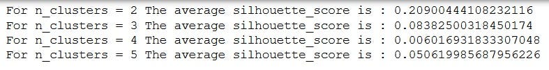
All results are close to 0, suggesting that the sample is on or very close to the decision boundary between two neighbouring clusters. In other words, there is no apparent indication of an underlying cluster structure in the dataset.

All results are close to 0, suggesting that the sample is on or very close to the decision boundary between two neighbouring clusters. In other words, there is no apparent indication of an underlying cluster structure in the dataset.

Both K-Means Elbow Method and Silhouette Analysis suggest that we cannot confirm an indication about the presence of the underlying cluster structure in the data set. It might be due to the characteristics of the city. Or it could be due to the quality of available data.

Both K-Means Elbow Method and Silhouette Analysis suggest that we cannot confirm an indication about the presence of the underlying cluster structure in the data set. It might be due to the characteristics of the city. Or it could be due to the quality of available data.

Whatever real reason it might be, all we know from these tuning results is that there is no convincing implication regarding the underlying cluster structure in the given data. In order to avoid an unreliable, and potentially misleading, recommendation, I would rather refrain from performing K-Means Clustering Model for the given dataset.

Whatever real reason it might be, all we know from these tuning results is that there is no convincing implication regarding the underlying cluster structure in the given data. In order to avoid an unreliable, and potentially misleading, recommendation, I would rather refrain from performing K-Means Clustering Model for the given dataset.

C. Discussion (C. Discussion)

C1. Three Lessons from Three Different Clustering Analyses (C1. Three Lessons from Three Different Clustering Analyses)

Lesson from the first objective:

Lesson from the first objective:

The first objective was to segregate outliers out of the dataset.

The first objective was to segregate outliers out of the dataset.

Before conducting clustering analysis, two simple boxplots automatically isolated outliers above their top whiskers from the rest: 8 in total for both of these two risk indices — the general security risk metric (Crime Severity Index) and the pandemic risk metric (COVID-19 Index).

Before conducting clustering analysis, two simple boxplots automatically isolated outliers above their top whiskers from the rest: 8 in total for both of these two risk indices — the general security risk metric (Crime Severity Index) and the pandemic risk metric (COVID-19 Index).

Then, DBSCAN clustering algorithm segmented these exactly identical 8 datapoints that the box plots identified as two remote clusters of sparsely distributed datapoints. Simply put, the machine learning model only confirmed the validity of the boxplots’ earlier automatic identification of those outliers.

Then, DBSCAN clustering algorithm segmented these exactly identical 8 datapoints that the box plots identified as two remote clusters of sparsely distributed datapoints. Simply put, the machine learning model only confirmed the validity of the boxplots' earlier automatic identification of those outliers.

This case tells us a lesson that a sophisticated method is not necessarily superior to a simpler method. Both of them did exactly the same job. We should take this lesson in modesty from the cost-benefit management perspective.

This case tells us a lesson that a sophisticated method is not necessarily superior to a simpler method. Both of them did exactly the same job. We should take this lesson in modesty from the cost-benefit management perspective.

Lesson from the second objective

Lesson from the second objective

The second objective was to segment ‘non-outlier’ neighbourhoods according to a compound risk metric (of CSS Index and COVID-19 Index).

The second objective was to segment 'non-outlier' neighbourhoods according to a compound risk metric (of CSS Index and COVID-19 Index).

The dendrogram of Hierarchical Clustering Model arranged 40 non-outlier neighbourhoods accordingly to their pairwise distance hierarchy. In other words, the dendrogram analysed and displayed the hierarchical structure of all the potential clusters automatically. And it allowed the user to explore and compare various cluster structures across different hierarchical levels. It’s worth running Hierarchical Clustering Model to generate the dendrogram because it visually helps the user shape human insight about the underlying cluster structural hierarchy. There is no other easier alternative to do the same job. It actually helped me to decide how many clusters to generate with Hierarchical Clustering algorithm for the second run.

The dendrogram of Hierarchical Clustering Model arranged 40 non-outlier neighbourhoods accordingly to their pairwise distance hierarchy. In other words, the dendrogram analysed and displayed the hierarchical structure of all the potential clusters automatically. And it allowed the user to explore and compare various cluster structures across different hierarchical levels. It's worth running Hierarchical Clustering Model to generate the dendrogram because it visually helps the user shape human insight about the underlying cluster structural hierarchy. There is no other easier alternative to do the same job. It actually helped me to decide how many clusters to generate with Hierarchical Clustering algorithm for the second run.

This presents a successful case that a machine learning model can play a productive role in supporting human decision-making process. A user can leverage one’s own profound domain expertise or human insight in the use of the dendrogram and effectively achieve the given objective.

This presents a successful case that a machine learning model can play a productive role in supporting human decision-making process. A user can leverage one's own profound domain expertise or human insight in the use of the dendrogram and effectively achieve the given objective.

The lesson here is that the user can proactively interact with machine learning algorithm to optimise the performance of machine learning and make a better decision.

The lesson here is that the user can proactively interact with machine learning algorithm to optimise the performance of machine learning and make a better decision.

Lesson from the third objective

Lesson from the third objective

The third objective was to cluster the neighbourhoods according to the Foursquare venue profile.

The third objective was to cluster the neighbourhoods according to the Foursquare venue profile.

I performed two hyperparameter tuning methods (K-Means Elbow Method and Silhouette Score Analysis) to discover the best n_clusters, one of the hyperparameters for K-Mean Clustering algorithm. Unfortunately, neither of them yielded a convincing implication about the underlying cluster structure in the Foursquare venue dataset. This suggests that a clustering model would unlikely yield a reliable result for the given dataset.

I performed two hyperparameter tuning methods (K-Means Elbow Method and Silhouette Score Analysis) to discover the best n_clusters , one of the hyperparameters for K-Mean Clustering algorithm. Unfortunately, neither of them yielded a convincing implication about the underlying cluster structure in the Foursquare venue dataset. This suggests that a clustering model would unlikely yield a reliable result for the given dataset.

The output of the machine learning is as good as the data input. The disappointing hyperparameter tuning result might have something to do with earlier concern about the quality of the Foursquare data.

The output of the machine learning is as good as the data input. The disappointing hyperparameter tuning result might have something to do with earlier concern about the quality of the Foursquare data.

Or, possibly there could be actually no particular underlying venue-based cluster structure among the neighbourhoods in CABA. That case, there would be no reason for running a clustering model for the dataset.

Or, possibly there could be actually no particular underlying venue-based cluster structure among the neighbourhoods in CABA. That case, there would be no reason for running a clustering model for the dataset.

Which is correct? This question, requiring a comparative study with data from other sources, might be a good topic for the second round of the study.

Which is correct? This question, requiring a comparative study with data from other sources, might be a good topic for the second round of the study.

Nonetheless, whatever real reason it might be, all I know from these tuning results is that there is no convincing implication regarding the underlying cluster structure in the given data. The lesson here would be: in the absence of supporting indication for the use of machine learning, I would be better off refraining from performing it in order to avoid a potentially misleading inference. Instead, I could rather provide more basic materials that can assist the Client use their human insight/domain expertise to analyse the subject.

Nonetheless, whatever real reason it might be, all I know from these tuning results is that there is no convincing implication regarding the underlying cluster structure in the given data. The lesson here would be: in the absence of supporting indication for the use of machine learning, I would be better off refraining from performing it in order to avoid a potentially misleading inference. Instead, I could rather provide more basic materials that can assist the Client use their human insight/domain expertise to analyse the subject.

Overall, with these different implications given, it would be na?ve to believe that we can simply automate machine learning process from the beginning to the end. Overall, all these cases support that human involvement could make machine learning more productive.

Overall, with these different implications given, it would be na?ve to believe that we can simply automate machine learning process from the beginning to the end. Overall, all these cases support that human involvement could make machine learning more productive.

C2. Suggestions for Future Development (C2. Suggestions for Future Development)

As the Client stressed at the outset of the project, this analysis was the preliminary analysis for a further extended study for their business expansion. Now, based on the findings from this analysis I would like to contribute some suggestions for the next round. Let me start.

As the Client stressed at the outset of the project, this analysis was the preliminary analysis for a further extended study for their business expansion. Now, based on the findings from this analysis I would like to contribute some suggestions for the next round. Let me start.

Different Local Source for Venue Data

Different Local Source for Venue Data

Unfortunately, for the second part of the third objective — to segment non-outlier neighbourhoods into clusters based on their venue profile — I could not derive any convincing inference regarding the underlying cluster structure among non-outlier neighbourhoods. There were two possibilities as aforementioned. As one possibility, there is some issue in the quality of the Foursquare data. As the other possibility, there is actually no underlying cluster structure in the actual subject.

Unfortunately, for the second part of the third objective — to segment non-outlier neighbourhoods into clusters based on their venue profile — I could not derive any convincing inference regarding the underlying cluster structure among non-outlier neighbourhoods. There were two possibilities as aforementioned. As one possibility, there is some issue in the quality of the Foursquare data. As the other possibility, there is actually no underlying cluster structure in the actual subject.

For the former case, I would suggest that the Client might benefit from exploring other sources than Foursquare to examine the venue profiles of these neighbourhoods. That would allow the Client to assess by comparison if the Foursquare data is representative of the actual state of popular venues in this particular city.

For the former case, I would suggest that the Client might benefit from exploring other sources than Foursquare to examine the venue profiles of these neighbourhoods. That would allow the Client to assess by comparison if the Foursquare data is representative of the actual state of popular venues in this particular city.

Furthermore, for the latter case, the Client might benefit from exploring other analysis than clustering in order to better understand the subject.

Furthermore, for the latter case, the Client might benefit from exploring other analysis than clustering in order to better understand the subject.

Different Scaling

Different Scaling

At the outset of the project, the Client specifically requested to scale risk metrics by ‘population density’. Nevertheless, it is not really clear whether ‘population density’ is the best feature for scaling. There are two other possible alternatives in the dataset: ‘area’ and ‘population’. An alternative scaling might yield a different picture about the risk profile of the neighbourhoods. For the second round of the study I would strongly suggest that the Client explore other scaling alternatives as well.

At the outset of the project, the Client specifically requested to scale risk metrics by 'population density'. Nevertheless, it is not really clear whether 'population density' is the best feature for scaling. There are two other possible alternatives in the dataset: 'area' and 'population'. An alternative scaling might yield a different picture about the risk profile of the neighbourhoods. For the second round of the study I would strongly suggest that the Client explore other scaling alternatives as well.

As a reminder, the characteristics of these three features’ data were presented at the stage of Data Understanding.

As a reminder, the characteristics of these three features' data were presented at the stage of Data Understanding.

Effective Data Science Project Management Policy Making

Effective Data Science Project Management Policy Making

At last, from the perspective of an effective Data Science project management, I would recommend that the Client should incorporate into their data analysis policy the following two lessons from this project.

At last, from the perspective of an effective Data Science project management, I would recommend that the Client should incorporate into their data analysis policy the following two lessons from this project.

1. When a basic tool can achieve the intended objective, it would be cost-effective to embrace it in deriving a conclusion/inference, rather than blindly implementing an advanced tool, such as machine learning.
   When a basic tool can achieve the intended objective, it would be cost-effective to embrace it in deriving a conclusion/inference, rather than blindly implementing an advanced tool, such as machine learning.
2. Unless we are certain that the given data is suitable for the design of a machine learning model — or whatever model, actually — it might be unproductive to run it. In such a case, there would be no point in wasting the precious resource to end up yielding a potentially misleading result.
   Unless we are certain that the given data is suitable for the design of a machine learning model — or whatever model, actually — it might be unproductive to run it. In such a case, there would be no point in wasting the precious resource to end up yielding a potentially misleading result.

Due to the hype for Machine Learning among the public, some clients demonstrate some blind craving for it, assuming that such an advanced tool would yield a superior result. Nevertheless, this project yielded a mixed set of answers of both ‘yes’ and ‘no’. Moreover, machine learning is not a panacea.

Due to the hype for Machine Learning among the public, some clients demonstrate some blind craving for it, assuming that such an advanced tool would yield a superior result. Nevertheless, this project yielded a mixed set of answers of both 'yes' and 'no'. Moreover, machine learning is not a panacea.

Especially since the Client demonstrated an exceptional enthusiasm towards Machine Learning for their future business decision making, I believe that it would be worthwhile reflecting these lessons in this report for their future productive conduct of data analysis.

Especially since the Client demonstrated an exceptional enthusiasm towards Machine Learning for their future business decision making, I believe that it would be worthwhile reflecting these lessons in this report for their future productive conduct of data analysis.

D. Final Products (D. Final Products)

Now, as the final products for this preliminary project, I decided to present the following summary materials — a pop-up Choropleth map, two scatter plots, and a summary table — that can help the Client use their domain expertise for their own analysis.

Now, as the final products for this preliminary project, I decided to present the following summary materials — a pop-up Choropleth map, two scatter plots, and a summary table — that can help the Client use their domain expertise for their own analysis.

D1. Pop Up Choropleth Map (D1. Pop Up Choropleth Map)

In order to summarize the results for all these objectives, I incorporated a pop-up feature into the choropleth map that I had created for the objective 1 and 2. Each pop-up would display the following additional information of the corresponding ‘non-outlier neighbourhood’.

In order to summarize the results for all these objectives, I incorporated a pop-up feature into the choropleth map that I had created for the objective 1 and 2. Each pop-up would display the following additional information of the corresponding 'non-outlier neighbourhood'.

• Name of the Neighbourhood
  Name of the Neighbourhood
• Cluster Risk Grade: to show ‘Centroid_Grade’, the cluster risk profile of the neighbourhood.
  Cluster Risk Grade: to show 'Centroid_Grade', the cluster risk profile of the neighbourhood.
• Top 3 Venue Categories
  Top 3 Venue Categories

The map below illustrates an example of the pop-up feature.

The map below illustrates an example of the pop-up feature.

For high risk ‘outlier neighbourhoods’, I controlled the pop-up feature, since the Client wants to exclude them from consideration.

For high risk 'outlier neighbourhoods', I controlled the pop-up feature, since the Client wants to exclude them from consideration.

As a precaution, the colour on the map represents the Risk Cluster, not the Venue Cluster. Since I refrained from generating Venue Cluster, there is no Venue Cluster information on the map. This map would allow the Client to explore the popular venue profile for each neighbourhood individually.

As a precaution, the colour on the map represents the Risk Cluster, not the Venue Cluster. Since I refrained from generating Venue Cluster, there is no Venue Cluster information on the map. This map would allow the Client to explore the popular venue profile for each neighbourhood individually.

D2. Scatter Plots (D2. Scatter Plots)

The following two scatter plots display the same underlying risk cluster structure: the first one with the names of neighbourhoods; the second without the names. In the first plot, the densely plotted names at the left bottom are obstructing the view of individual datapoints (‘non-outlier neighbourhoods’) in the first plot. In the second one without the name, the entire view of the cluster structure can be seen clearly.

The following two scatter plots display the same underlying risk cluster structure: the first one with the names of neighbourhoods; the second without the names. In the first plot, the densely plotted names at the left bottom are obstructing the view of individual datapoints ('non-outlier neighbourhoods') in the first plot. In the second one without the name, the entire view of the cluster structure can be seen clearly.

Top 5 Popular Summary (Top 5 Popular Summary)

In addition, I also include a summary table to present the top 5 popular venue categories for each neighbourhood, sorted by the cluster’s risk profile (in ascending order of Centroid_Grade) and the number of Foursquare venue response (in descending order of Venue Response). In this sorted order, the Client can view the list of neighbourhoods in the following manner: from the safest cluster to more risker ones; from presumably the commercially busiest neighbourhood to less busier ones.

In addition, I also include a summary table to present the top 5 popular venue categories for each neighbourhood, sorted by the cluster's risk profile (in ascending order of Centroid_Grade) and the number of Foursquare venue response (in descending order of Venue Response). In this sorted order, the Client can view the list of neighbourhoods in the following manner: from the safest cluster to more risker ones; from presumably the commercially busiest neighbourhood to less busier ones.

Since the table is very long, here I would present only the top 7 rows of the table.

Since the table is very long, here I would present only the top 7 rows of the table.

That’s all about my very first Data Science Capstone Project.

That's all about my very first Data Science Capstone Project.

Thank you very much for reading through this article.

Thank you very much for reading through this article.

Michio Suginoo

Michio Suginoo