Continuing from the seventh article in this series, we are going to explore ways to present data. Over the past few years, Marketing and SEO field has become more data-driven than in the past thanks to tools like Google Webmaster Tools and Google Analytics, Majestic SEO, SEMRush, and few others. So, presenting data is something every SEO & Marketing guy should know. This article covers how to present data.

C來自ontinuing 在本系列的十七條 ，我們要探索的方式來呈現數據。 在過去的幾年中，得益于Google網站站長工具和Google Analytics(分析)，Majestic SEO，SEMRush等工具，“營銷”和“ SEO”領域已變得比過去更受數據驅動。 因此，呈現數據是每個SEO和營銷人員都應該知道的。 本文介紹如何呈現數據。

呈現數據 (PRESENTING DATA)

適用于營銷人員的Excel和表格-創建有意義的報告，為您的客戶提供強大的見解 (Excel and Sheets for marketers — create meaningful reports that provides strong insights to your customers)

Clients have become wiser and they want reliable SEO advice with a strong verifiable foundation. Many SEO guys are now finding themselves faced with the task of doing fairly complex data analysis to improve their search strategies, and Excel adequacy is not quite enough. In this article, we will be including real-world SEO tasks, ranging from the relatively simple to rather complex. So, if Sorting and filtering data, SUM functions, Count Commands, Pivot tables, Vlookup tables, Index Match & Conditional Formatting make you scratch your head, then read on.

客戶變得更加明智，他們希望在可驗證的基礎上獲得可靠的SEO建議。 現在，許多SEO專家正面臨著進行相當復雜的數據分析以改善其搜索策略的任務，而Excel的充分性還不夠。 在本文中，我們將包括從相對簡單到相當復雜的實際SEO任務。 因此，如果對數據進行排序和篩選，SUM函數，計數命令，數據透視表，Vlookup表，索引匹配和條件格式設置使您抓狂，然后繼續閱讀。

NOTE: Majority of the online digital analytics courses starts and ends at Google Analytics. Very few teaches how to probe & present data meaningfully using Google Sheets/Excel, Google Data Studio & Big Query.

注意：大多數在線數字分析課程都是在Google Analytics(分析)開始和結束的。 很少有人教如何使用Google Sheets / Excel，Google Data Studio和Big Query有意義地探查和呈現數據。

CXL’s Excel and Sheets for marketers by Fred Pike is one such course. This Institute aims at building advanced level data-driven marketing skills.

弗雷德·派克 ( Fred Pike) 為營銷人員設計的CXL Excel和表格 就是其中一門課程。 該研究所旨在培養高級的數據驅動型營銷技能。

In this article, we are going to cover the following topics. A single article cannot cover them comprehensively. But if mastered properly, these tricks will make life easier for any SEO and Marketing guy.

在本文中，我們將介紹以下主題。 一篇文章無法全面介紹它們。 但是，如果掌握得當，這些技巧將使任何SEO和市場營銷人員的工作更加輕松。

排序和過濾數據： (Sort and Filter data:)

At some point in your life, as an analyst or digital marketer, you’re going to download data and sort it intelligently.

在您生活中的某個時刻，作為分析師或數字營銷人員，您將下載數據并進行智能排序。

Sorting is a common spreadsheet task that allows you to easily reorder your data. The most common type of sorting is alphabetical ordering, which you can do in ascending or descending order.

排序是一項常見的電子表格任務，可讓您輕松地對數據進行重新排序。 最常見的排序類型是字母排序，您可以按升序或降序進行排序。

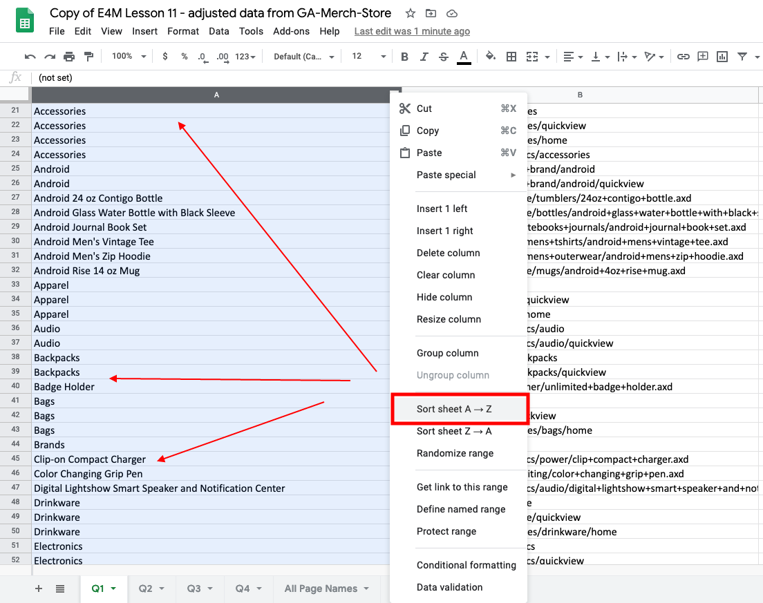
Filtering limits the visibility of a table’s content to only those entries that match the criteria specified in the filter. To perform a filtering operation on a range of cells, select any cell in that range and click on the Filter button. You will find it in the specific header row top right. Once clicked, it will show you various options to sort data like shown in the example. Here we have sorted a lot of data that is limited to Bags and Accessories only.

過濾將表內容的可見性限制為僅與過濾器中指定的條件匹配的那些條目。 要對一系列單元格執行過濾操作，請選擇該范圍內的任何單元格，然后單擊“過濾器”按鈕。 您會在右上方的特定標題行中找到它。 單擊后，它將顯示如示例中所示的各種數據排序選項。 在這里，我們對很多數據進行了排序，這些數據僅限于箱包和配件。

SUM功能-它包含三個重要功能： (SUM Functions- It contains three vital functions:)

1. SUM (sums everything)

   總和(總和)

The SUM function adds values. You can add individual values, cell references or ranges or a mix of all three. It is also called the Auto Sum function.

SUM函數可添加值。 您可以添加單個值，單元格引用或范圍，也可以添加所有三個值的組合。 也稱為自動求和功能。

For example:

例如：

• =SUM(A2:A10) Adds the values in cells A2:10.

  = SUM(A2：A10)將單元格A2：10中的值相加。

• =SUM(A2:A10, C2:C10) Adds the values in cells A2:10, as well as cells C2:C10.

  = SUM(A2：A10，C2：C10)將單元格A2：10和單元格C2：C10中的值相加。

2. SUMIF (sums based on one condition)

2. SUMIF(基于一種條件的總和)

You use the SUMIF function to sum the values in a range that meet criteria that you specify. For example, suppose that in a column that contains numbers, you want to sum only the values that are larger than 5. You can use the following formula: =SUMIF(B2:B25,”>5")

您可以使用SUMIF函數對滿足指定條件的范圍內的值求和。 例如，假設在一個包含數字的列中，您只希望對大于5的值求和。可以使用以下公式： = SUMIF(B2：B25，“> 5”)

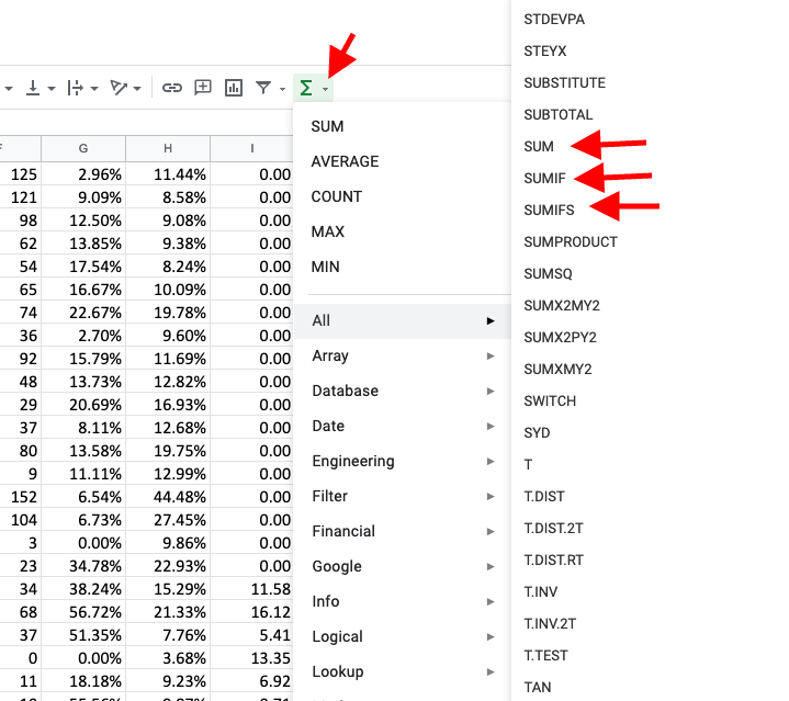
3. SUMIFS (sums based on multiple conditions)

3. SUMIFS(基于多個條件的總和)

The SUMIFS function adds all of its arguments that meet multiple criteria. For example, you may use SUMIFS to sum the number of retailers in the country who (1) reside in a single zip code and (2) whose profits exceed a specific dollar value.

SUMIFS函數添加其滿足多個條件的所有參數。 例如，您可以使用SUMIFS來匯總該國家/地區的零售商數量，這些零售商(1)居住在單個郵政編碼中，(2)利潤超過特定的美元價值。

• SUMIFS(sum_range, criteria_range1, criteria1, [criteria_range2, criteria2], …)

  SUMIFS(sum_range，criteria_range1，criteria1，[criteria_range2，criteria2]，...)

計數命令 (Count Commands)

1. Count (counts the number of numeric items)

   計數(計算數字項的數量)

The COUNT function counts the number of cells that contain numbers and counts numbers within the list of arguments. Use the COUNT function to get the number of entries in a number field that is in a range or array of numbers.

COUNT函數計算包含數字的單元格的數量，并計算參數列表中的數字。 使用COUNT函數可獲取數字范圍或數字數組中的條目數。

2. Counta (counts the number of text items)

2. Counta(計算文本項的數量)

The COUNTA function also counts cells containing any type of information, including error values and empty text (“”). For example, if the range contains a formula that returns an empty string, the COUNTA function counts that value.

COUNTA函數還計算包含任何類型的信息的單元格，包括錯誤值和空文本(“”)。 例如，如果范圍包含返回空字符串的公式，則COUNTA函數將對該值進行計數。

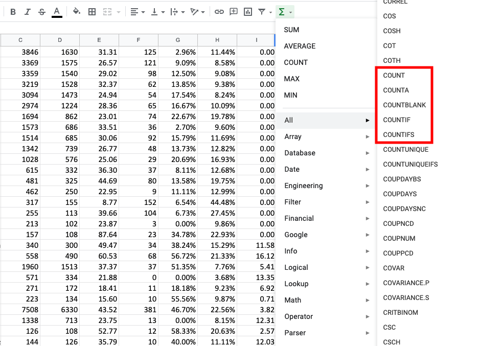
3. CountIF (counts based on one condition)

3. CountIF(基于一種條件的計數)

Use COUNTIF to count the number of cells that meet a criterion; for example, to count the number of times a particular city appears in a customer list.

使用COUNTIF計數符合條件的單元格數量； 例如，計算特定城市出現在客戶列表中的次數。

In its simplest form, COUNTIF says:

COUNTIF最簡單的形式是：

• =COUNTIF(Where do you want to look?, What do you want to look for?)
  = COUNTIF(您想去哪里？，您想尋找什么？)

4. CountIFS (counts based on multiple conditions)

4. CountIFS(基于多個條件的計數)

The COUNTIFS function applies criteria to cells across multiple ranges and counts the number of times all criteria are met.

COUNTIFS函數將標準應用于多個范圍的單元格，并計算滿足所有條件的次數。

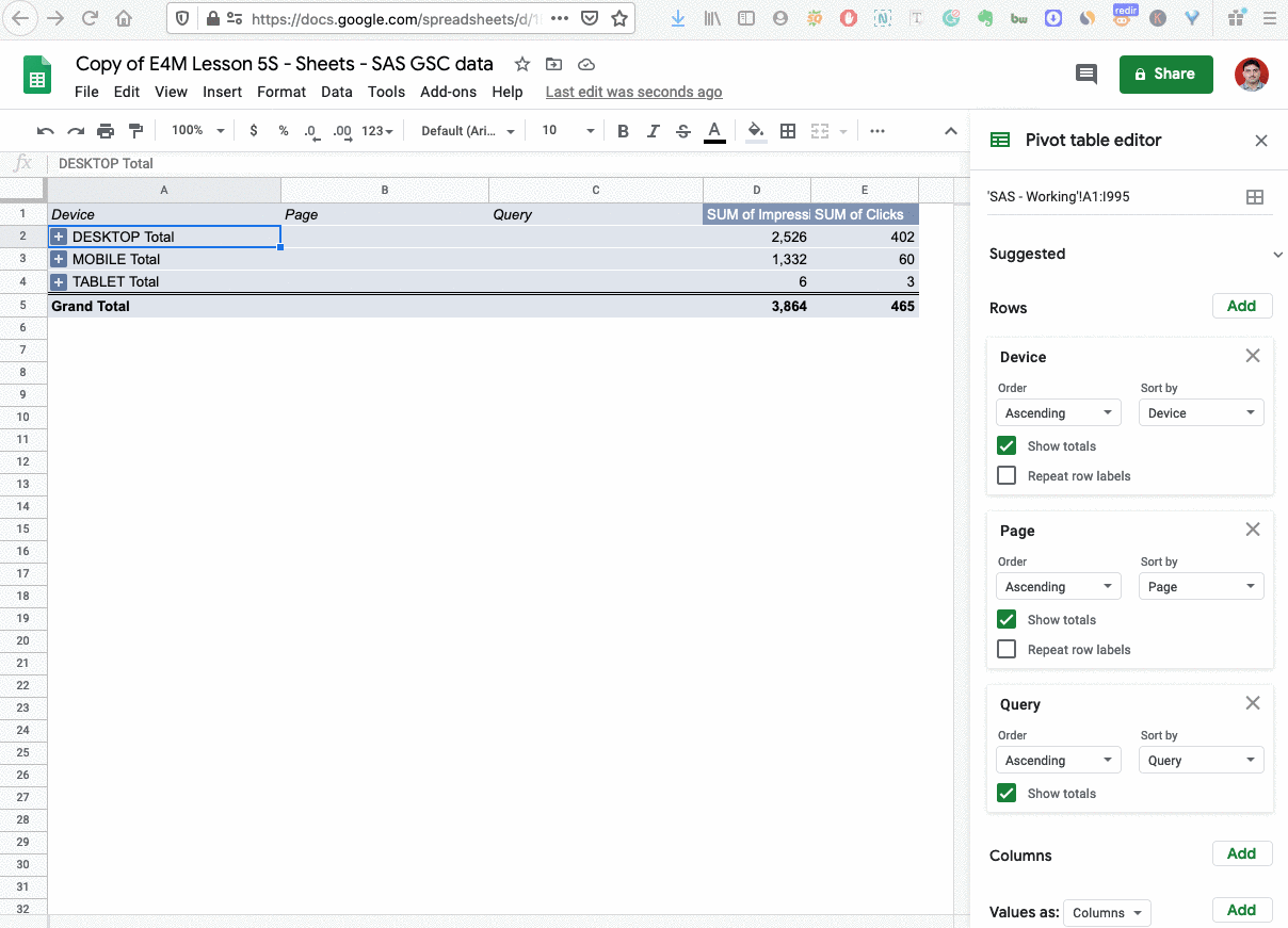
數據透視表 (Pivot Tables)

Once you’ve got all of your data calculated and properly formatted then now it’s time to analyze it all and build an action plan. Surely, this can be done without the use of pivot tables and charts, but this powerful feature can make it a much easier process.

計算完所有數據并正確格式化后，現在該對所有數據進行分析并制定行動計劃了。 當然，無需使用數據透視表和圖表即可完成此操作，但是此強大的功能可以使其變得更加輕松。

The Pivot tables are Excel’s one of the most powerful tool. It helps you drill down deep into numerical data and see unanticipated scenarios. This will help you make better-informed decisions. It helps you summarize and analyze data, see comparisons, patterns and trends both in tabular form as well as in Pivot Chart reports.

數據透視表是Excel最強大的工具之一。 它可以幫助您深入研究數字數據并查看意外情況。 這將幫助您做出更明智的決策。 它可以幫助您匯總和分析數據，以表格形式以及在“數據透視圖”報告中查看比較，模式和趨勢。

To create a pivot table you need to have your data source ready first. This could be in the form of an Excel table, a range of cells that contains the data you require, or an external data source like an Access database.

要創建數據透視表，您需要首先準備好數據源。 這可以采用Excel表，包含所需數據的單元格范圍或外部數據源(如Access數據庫)的形式。

To create a pivot table using Sheets, click anywhere inside your source data, select Data from the menu and then pivot table. It is always better to create a pivot table instead of a pivot chart. This will give a better idea of how your data looks and you can fine-tune your data view before making the charts. The chart option is useful when you are ready with your data and you are certain about how your Pivot Table should be.

要使用表格創建數據透視表，請在源數據內的任意位置單擊，從菜單中選擇數據，然后再選擇數據透視表。 創建數據透視表而不是數據透視表總是更好。 這樣可以更好地了解數據的外觀，并且可以在制作圖表之前微調數據視圖。 當您準備好數據并確定數據透視表應如何時，圖表選項很有用。

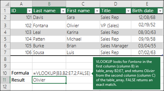
Vlookup (Vlookup)

The purpose of Vlookup is to help you find a single piece of information in a table based on a single criterion.

Vlookup的目的是幫助您基于單個條件在表中查找單個信息。

Microsoft Excel Definition: Looks for a value in the leftmost column of a table, and then returns a value in the same row from a column you specify. By default, the table must be sorted in an ascending order.

Microsoft Excel定義：在表的最左列中查找一個值，然后從您指定的列的同一行中返回一個值。 默認情況下，表必須按升序排序。

Let us say you have downloaded a client list from your CRM and it contains data in the form of Client IDs, addresses, phone numbers, and open balance amount. If you need to pull data from the original client list into another sheet, VLOOKUP can help you build this system dynamically by pulling information.

假設您已經從CRM中下載了一個客戶列表，其中包含客戶ID，地址，電話號碼和未結余額金額形式的數據。 如果您需要將數據從原始客戶端列表中拉到另一個工作表中，VLOOKUP可以通過拉信息來幫助您動態構建該系統。

Another example, Use VLOOKUP when you need to find things in a table or a range by row. For example, look up the price of an automotive part by the part number, or find an employee name based on their employee ID.

另一個示例是，當您需要在表或行范圍中查找內容時，請使用VLOOKUP。 例如，通過零件編號查找汽車零件的價格，或根據員工的ID查找員工的姓名。

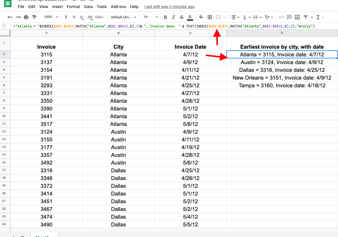
索引匹配 (INDEX MATCH)

INDEX MATCH is a set of functions nested together that essentially performs the same task that VLOOKUP does, except it does it a little differently (and more efficiently).

INDEX MATCH是一組嵌套在一起的函數，它們基本上執行與VLOOKUP相同的任務，只是它的執行方式略有不同(且效率更高)。

This formula is popular among the most elite Excel users because it offers some advantages over the VLOOKUP. This formula is a combination of the INDEX and MATCH functions.

該公式在大多數Excel精英用戶中都很流行，因為它比VLOOKUP具有一些優勢。 此公式是INDEX和MATCH函數的組合。

This example below employs the INDEX and MATCH functions together to return the earliest invoice number and its corresponding date for each of five cities. Because the date is returned as a number, we use the TEXT function to format it as a date.

下面的示例使用INDEX和MATCH函數一起返回五個城市中每個城市的最早發票編號及其對應的日期。 因為日期以數字形式返回，所以我們使用TEXT函數將其格式化為日期。

條件格式 (Conditional formatting)

Conditional formatting is one of the areas of excel that can be especially useful when building reports for upper management or your clients by allowing you the ability to make formatting changes automatically to any cell depending different conditions.

條件格式設置是excel的擅長領域之一，因為它使您能夠根據不同的條件自動對任何單元格進行格式更改，從而在為高層管理人員或客戶構建報告時特別有用。

Being able to present data in clean, easy to understand manner is part of creating effective reports but it’s so often overlooked. Conditional formatting not only makes things easier on you to highlight important data points, but it does it in a way that can be automated and scales with your data.

能夠以簡潔，易于理解的方式呈現數據是創建有效報告的一部分，但它經常被忽略。 條件格式不僅使您可以輕松地突出顯示重要的數據點，而且可以自動實現并隨數據縮放的方式。

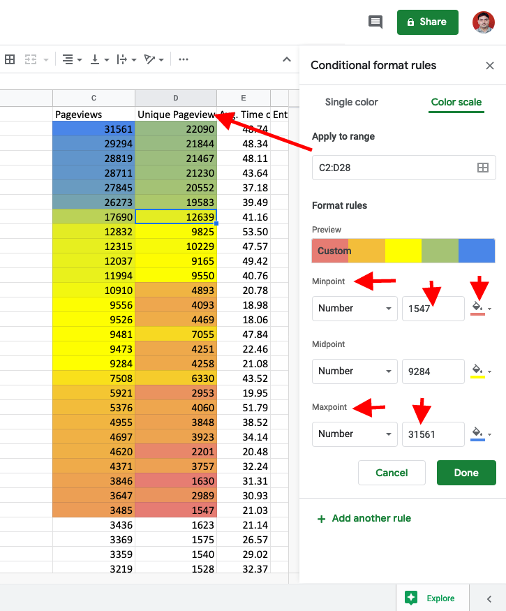
Use conditional formatting to help you visually explore and analyze data, detect critical issues, and identify patterns and trends.

使用條件格式設置可以幫助您直觀地瀏覽和分析數據，檢測關鍵問題以及確定模式和趨勢。

Conditional formatting makes it easy to highlight interesting cells or ranges of cells, emphasize unusual values, and visualize data by using data bars, color scales, and icon sets that correspond to specific variations in the data.

使用條件格式設置，可以輕松突出顯示感興趣的單元格或單元格范圍，強調不尋常的值以及通過使用與數據的特定變體相對應的數據欄，色標和圖標集來可視化數據。

迷你圖 (Sparklines)

Sparklines are pretty easy to add and they add a little bit of pizzazz and colour to the spreadsheet. They’re a nice little tool to have in your tool belt.

迷你圖非常容易添加，并且會在電子表格中添加一點點陰影和顏色。 它們是您工具帶中不錯的小工具。

A sparkline is a tiny chart in a worksheet cell that provides a visual representation of data. Use sparklines to show trends in a series of values, such as seasonal increases or decreases, economic cycles, or to highlight maximum and minimum values. Position a sparkline near its data for greatest impact.

迷你圖是工作表單元格中的一個很小的圖表，可提供數據的可視化表示。 使用迷你圖顯示一系列值的趨勢，例如季節性增加或減少，經濟周期，或突出顯示最大值和最小值。 將迷你圖放置在其數據附近以產生最大影響。

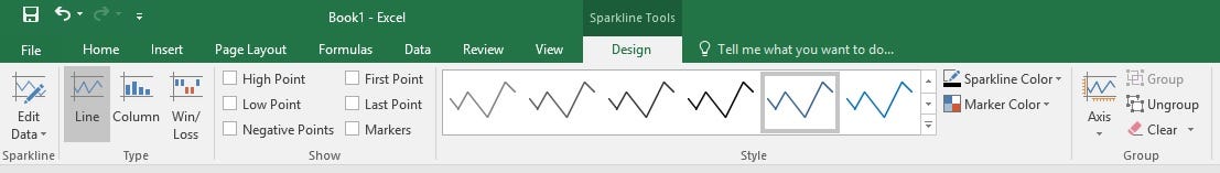
The way we do that in Excel is through the insert command. You see, there’s a Sparkline section here, and you have different options for what type of graph to insert. There are three different types of sparklines: Line, Column, and Win/Loss. Line and Column work the same as line and column charts. Win/Loss is similar to Column, except it only shows whether each value is positive or negative instead of how high or low the values are.

我們在Excel中執行此操作的方法是通過insert命令。 您會看到，這里有一個迷你圖部分，對于要插入的圖形類型，您有不同的選擇。 迷你圖有三種不同類型：線條， 列和贏/虧。 的行和列的工作相同的行和列圖表。 贏/虧與Column相似，不同之處在于它僅顯示每個值是正數還是負數，而不顯示值的高低。

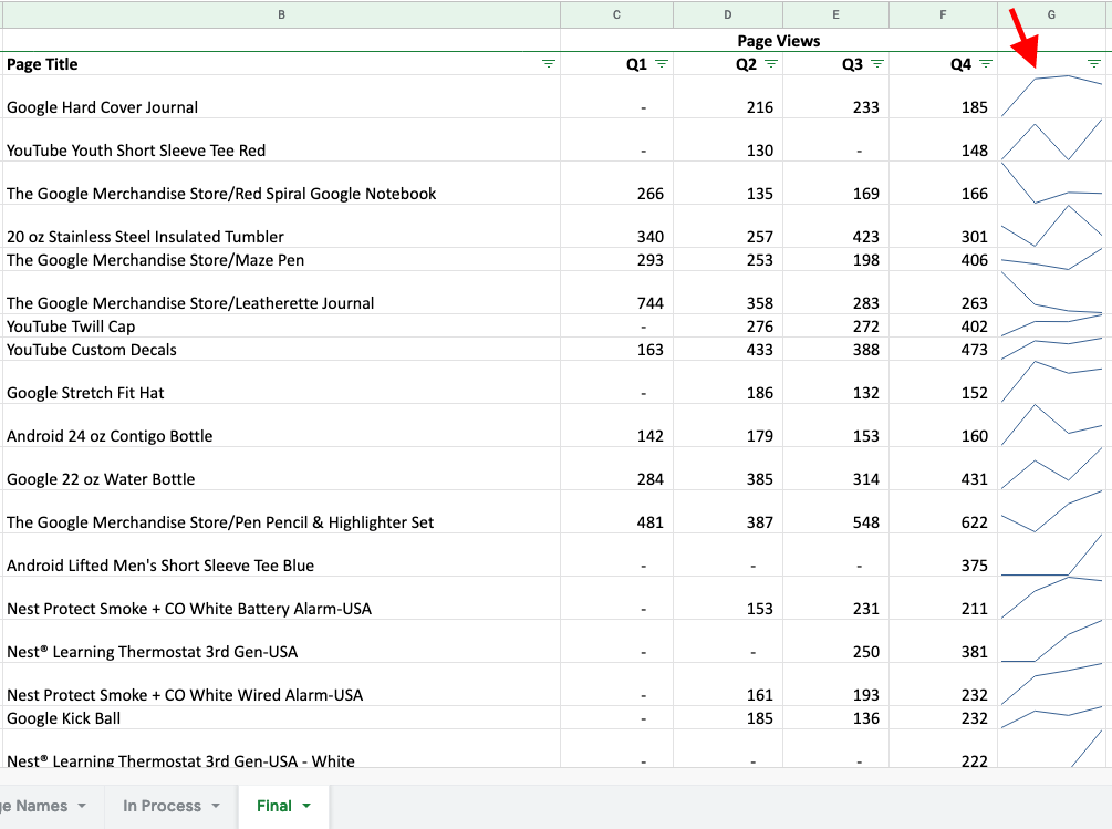
Now you already know, creating sparklines in Excel is easy and straight forward. Sparklines can only be used in Excel 2010 and later; in Excel 2007 and earlier, they are not shown.

現在您已經知道，在Excel中創建迷你圖很簡單。 迷你圖只能在Excel 2010和更高版本中使用； 在Excel 2007及更早版本中，它們不會顯示。

In the next article, we will Learn to create impressive, insightful & time-saving reports with Google Data Studio

在下一篇文章中，我們將學習如何使用 Google Data Studio 創建令人印象深刻，見解深刻且節省時間的報告

CXL Institute is the only skill-building platform for marketers that uses the world’s top 1% practitioners as instructors. I have gone through a lot of video course before but I have never enjoyed my learning journey like I have with this course. The depth that is provided by this course and how it can shape up your career from your current position to a Digital Analytics Guy is amazing.

CXL研究所 是針對營銷人員的唯一技能培養平臺，該平臺使用了全球排名前1％的從業人員作為指導。 我之前已經學過很多視頻課程，但是從未像過這門課程那樣享受學習的樂趣。 這門課程提供的深度知識以及它如何從您目前的職位發展到Digital Analytics Guy，可以塑造您的職業生涯。