介紹 (Introduction)

Bayesian analysis offers the possibility to get more insights from your data compared to the pure frequentist approach. In this post, I will walk you through a real life example of how a Bayesian analysis can be performed. I will demonstrate what may go wrong when choosing a wrong prior and we will see how we can summarize our results. For you to follow this post, I assume you are familiar with the foundations of Bayesian statistics and with Bayes' theorem.

與純頻率論方法相比，貝葉斯分析提供了從數據中獲得更多見解的可能性。 在本文中，我將向您介紹如何執行貝葉斯分析的真實示例。 我將演示選擇錯誤的先驗時可能出問題的地方，我們將看到如何總結我們的結果。 為了讓您關注這篇文章，我假設您熟悉貝葉斯統計的基礎和貝葉斯定理。

情境 (Scenario)

As an example analysis, we will discuss a real life problem from a physics lab. No worries, you don't need any physics knowledge for that. We want to determine the efficiency of a particle detector. A particle detector is a sensor that may produce a measurable signal when certain particles traverse it. The efficiency of the detector we want to evaluate is the chance that the detector actually measures the traversing particle. In order to measure this, we put the detector that we want to evaluate in between two other sensors in a sandwich-like structure. If we measure a signal in the top and bottom sensors we know that a particle should have also traversed the detector in the middle. A picture of the experimental setup is shown below.

作為示例分析，我們將討論物理實驗室中的現實生活中的問題。 不用擔心，您不需要任何物理知識。 我們要確定粒子探測器的效率。 粒子檢測器是一種傳感器，當某些粒子經過時會產生可測量的信號。 我們要評估的檢測器效率是檢測器實際測量橫越粒子的機會。 為了對此進行測量，我們將要評估的檢測器放在其他兩個傳感器之間，呈三明治狀。 如果我們在頂部和底部傳感器中測量信號，我們知道粒子也應該在中間穿過檢測器。 實驗設置的圖片如下所示。

For the measurement, we count the number of traversing particles N in a certain time (as reported by the top and bottom sensors) as well as the number of signals measured in our detector r. For this example, we assume N=100 and r=98.

為了進行測量，我們計算了一定時間內(由頂部和底部傳感器報告的)遍歷粒子N的數量，以及在探測器r中測得的信號數量。 對于此示例，我們假設N = 100和r = 98 。

頻頻結果 (Frequentist Result)

In a frequentist approach, we could use our measured data and arrive at the conclusion that the efficiency of the detector is e = r/N = 98%. This gives us only a point estimate. If we want to answer more complicated questions, for example: "What is the probability that the efficiency of the detector is above 99%", then we need a more complex analysis.

在常用方法中，我們可以使用我們的測量數據得出結論，即探測器的效率為e = r / N = 98％ 。 這僅給我們一個點估計。 如果我們想回答更復雜的問題，例如： “檢測器的效率高于99％的概率是多少” ，那么我們需要進行更復雜的分析。

貝葉斯分析 (The Bayesian Analysis)

The goal of the Bayesian approach is to derive the full posterior probability distribution of the efficiency of the detector given our data p(e|D). In order to do so, we need Bayes' theorem:

貝葉斯方法的目標是在給定我們的數據p(e | D)的情況下 ，得出探測器效率的全部后驗概率分布。 為此，我們需要貝葉斯定理：

We will go over the different terms in the following.

下面我們將討論不同的術語。

概率模型/可能性： p(D | e) (Probability Model / Likelihood: p(D|e))

As always in a Bayesian analysis, we need to select a model that describes the process we want to analyse, called the likelihood. For our problem, we can interpret the efficiency as the chance to have a success (r) out of a certain number of trails (N). This class of problems, similar to determining the chance of a coin showing head, can be modeled by the binomial distribution:

與貝葉斯分析一樣，我們需要選擇一個模型來描述我們要分析的過程，即可能性。 對于我們的問題，我們可以將效率解釋為從一定數量的線索( N )中獲得成功( r )的機會。 此類問題類似于確定硬幣出現正面的機會，可以通過二項分布來建模：

先前：p(e) (Prior: p(e))

Next, we need to define a prior. Here, we start with the most trivial choice, a flat prior. We will discuss the influence of a different prior choice later.

接下來，我們需要定義一個先驗。 在這里，我們從最簡單的選擇開始，即優先選擇。 稍后，我們將討論不同的優先選擇的影響。

邊際可能性：p(D) (Marginal Likelihood: p(D))

The marginal likelihood is the denominator in Bayes' theorem. Luckily it is just a normalization constant and not dependent on the efficiency. We can determine it numerical by finding the constant that normalizes the posterior to 1.

邊際可能性是貝葉斯定理中的分母。 幸運的是，這只是一個歸一化常數，與效率無關。 我們可以通過找到將后驗歸一化為1的常數來確定它的數值。

結果 (Results)

Now we can calculate the posterior following Bayes' theorem.

現在我們可以計算遵循貝葉斯定理的后驗。

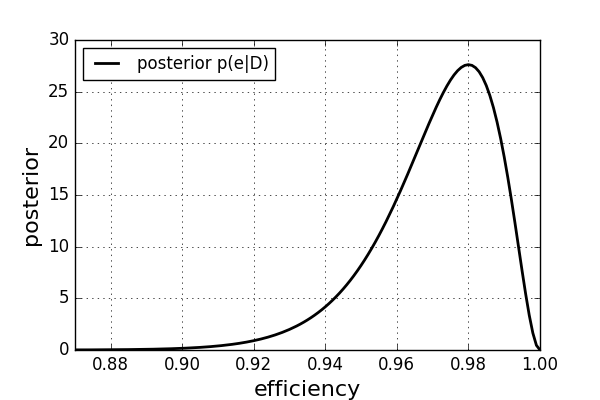
You can see that the most probable value is e=98% which is the same as the intuitive frequentist result. But we obtained much more information here, as we got the full posterior probability distribution. For example, we can see that the distribution is asymmetric. An efficiency below 97% has a higher probability than an efficiency above 99%. And to both probabilities, we can assign exact numbers. How did we get this extra information? It is because we took advantage of more information, meaning we have assumed that the behaviour of the detector follows a binomial distribution as well as we assumed a flat prior distribution.

您可以看到最可能的值是e = 98％ ，這與直觀的常客結果相同。 但是，由于獲得了完整的后驗概率分布，我們在這里獲得了更多的信息。 例如，我們可以看到分布是不對稱的。 低于97％的效率比高于99％的效率更高的概率。 對于這兩種概率，我們可以分配確切的數字。 我們如何獲得這些額外信息？ 這是因為我們利用了更多的信息，這意味著我們假設檢測器的行為遵循二項式分布，并且假設了先驗分布平坦。

先驗的影響 (Influence of the Prior)

The prior plays an important role in a Bayesian analysis. In the following, we will see what happens if we change it. Let’s say we find a statement in the datasheet of the detector that the efficiency can be assumed to be gaussian distributed around 98% with a standard deviation of s=1%. In an older version of the datasheet, however, we find that the efficiency of the detector should be Gaussian distributed around 92% with the same standard deviation of s=1%. We incorporate this information into the posterior by changing the priors accordingly. The results for both cases can be seen below.

先驗在貝葉斯分析中起重要作用。 在下面，我們將看到如果更改它會發生什么。 假設我們在檢測器的數據表中找到一條陳述，即效率可以假定為高斯分布，其標準偏差為s = 1％，約為98 ％ 。 但是，在數據表的舊版本中，我們發現檢測器的效率應為高斯分布，約為92％，且標準偏差為s = 1％ 。 我們通過相應地更改先驗將這些信息合并到后驗中。 這兩種情況的結果都可以在下面看到。

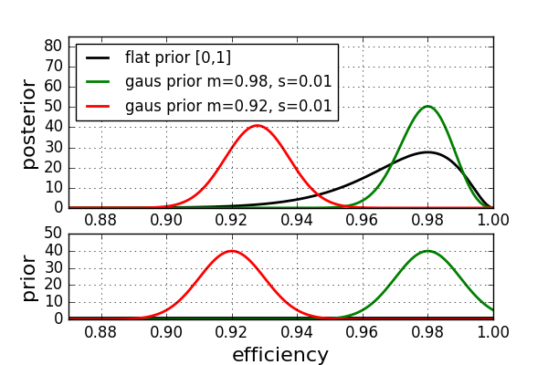
Here, the posterior is shown in the top panel and the corresponding priors in the panel below. The black curve shows the previous result with the flat prior. When changing the prior to a gaussian one with mean m=98% (green) the posterior peaks again at 98% and the confidence in our estimates are stronger compared to the case with the flat prior. The prior supports our data. While an efficiency below 95% still had a reasonable probability in the case of the flat prior, it is nearly excluded now. Taking the prior from the old data sheet that peaked at an efficiency of 92% (red), we can see that the posterior differs significantly from the other two. The most probable value is around 93%, completely changing our results. How can this be? The problem is that by choosing a wrong prior the data and the prior are not consistent with each other. This example shows, that choosing a wrong prior may have catastrophic consequences. It is important to always evaluate the consistency between the prior, the probability model and the posterior.

在這里，后部顯示在頂部面板中，而相應的先驗顯示在下方面板中。 黑色曲線顯示先前的結果，平坦的先驗結果。 當將先驗者轉換為均值m = 98％ (綠色)的高斯驗算器時，后驗峰再次以98％的峰值出現，并且與持平先驗者相比，我們的估計信心更大。 先驗支持我們的數據。 而效率低于 在之前持平的情況下，仍有95％的人具有合理的可能性，現在幾乎將其排除在外。 從舊數據表中的先驗數據以92％(紅色)的效率達到峰值，我們可以看到，后驗數據與其他兩個數據表明顯不同。 最可能的值約為93％，完全改變了我們的結果。 怎么會這樣？ 問題在于，通過選擇錯誤的先驗，數據和先驗數據彼此不一致。 此示例表明，選擇錯誤的先驗可能會帶來災難性的后果。 始終評估先驗概率模型和后驗模型之間的一致性很重要。

合并其他度量 (Incorporating Additional Measurements)

Another use case for a prior is an additional measurement. Imagine your colleague measured the same detector. He measured N1=300 and r1=280. How can we correctly make use of this data? We can use it as a prior for our analysis. The results are shown below.

先驗的另一個用例是額外的度量。 想象一下您的同事測量了相同的檢測器。 他測得N1 = 300和r1 = 280 。 我們如何正確利用這些數據？ 我們可以將其用作分析的先驗條件。 結果如下所示。

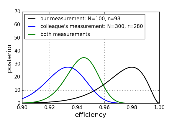
You can see the posterior distribution of our measurement (black) and the colleague's measurement (blue) both using flat priors. If we use our colleague's measurement as a prior for our analysis, we arrive at the green curve. The most probable value of the green curve is in between the other two curves, but more shifted to the blue curve as our colleague's measurement has more data. Also, the distribution for the green curve is slightly narrower compared to the other two. Side note: The resulting posterior is again a binomial distribution. Moreover, we will arrive at the same posterior as if we would redo the analysis and assume only one measurement with N=N1+N2=400 and r=r1+r2=378. As you would expect it, the results are also independent of the order the two measurements were performed. This can be easily verified analytically.

您可以使用平坦先驗值來查看我們的度量的后驗分布(黑色)和同事的度量(藍色)。 如果我們將同事的測量結果作為分析的先驗條件，則會得出綠色曲線。 綠色曲線的最可能值在其他兩條曲線之間，但是隨著我們同事的測量結果具有更多數據，更多地轉移到了藍色曲線。 此外，綠色曲線的分布比其他兩條曲線略窄。 旁注 ：產生的后驗再次是二項分布。 此外，我們將得出相同的后驗，就好像我們要重做分析并假設只有一個測量值N = N1 + N2 = 400且r = r1 + r2 = 378一樣 。 如您所料，結果也與兩次測量的執行順序無關。 可以很容易地進行分析驗證。

如何呈現結果 (How to present your results)

After calculating the posterior, we now want to present our results. Ideally, you want to show the full posterior distribution, as this reflects the full information. However, this is not always possible and you may want to summarize it with a set of values. Often you want to give a point estimate along with an interval that summarizes the width of the distribution. There are different ways how to do this. Popular choices include:

在計算后驗后，我們現在要展示我們的結果。 理想情況下，您希望顯示完整的后驗分布，因為這反映了完整的信息。 但是，這并非總是可能的，您可能需要用一組值對其進行總結。 通常，您需要給出一個點估計值以及一個總結分布寬度的間隔。 有不同的方法來執行此操作。 受歡迎的選擇包括：

• Expectation value & standard deviation
  期望值和標準偏差
• Median & central interval
  中位和中心間隔
• Mode & smallest interval
  模式和最小間隔

Additionally, we need to select how much probability should be included in the intervals (often used: 68% or 90%).

此外，我們需要選擇在間隔中應包含多少概率(通常使用：68％或90％)。

For a normal distribution, all three choices of point estimate and confidence interval give identical results. However, in our case of a skewed distribution this is not the case.

對于正態分布，點估計和置信區間的所有三個選擇都給出相同的結果。 但是，在我們的分布偏斜的情況下，情況并非如此。

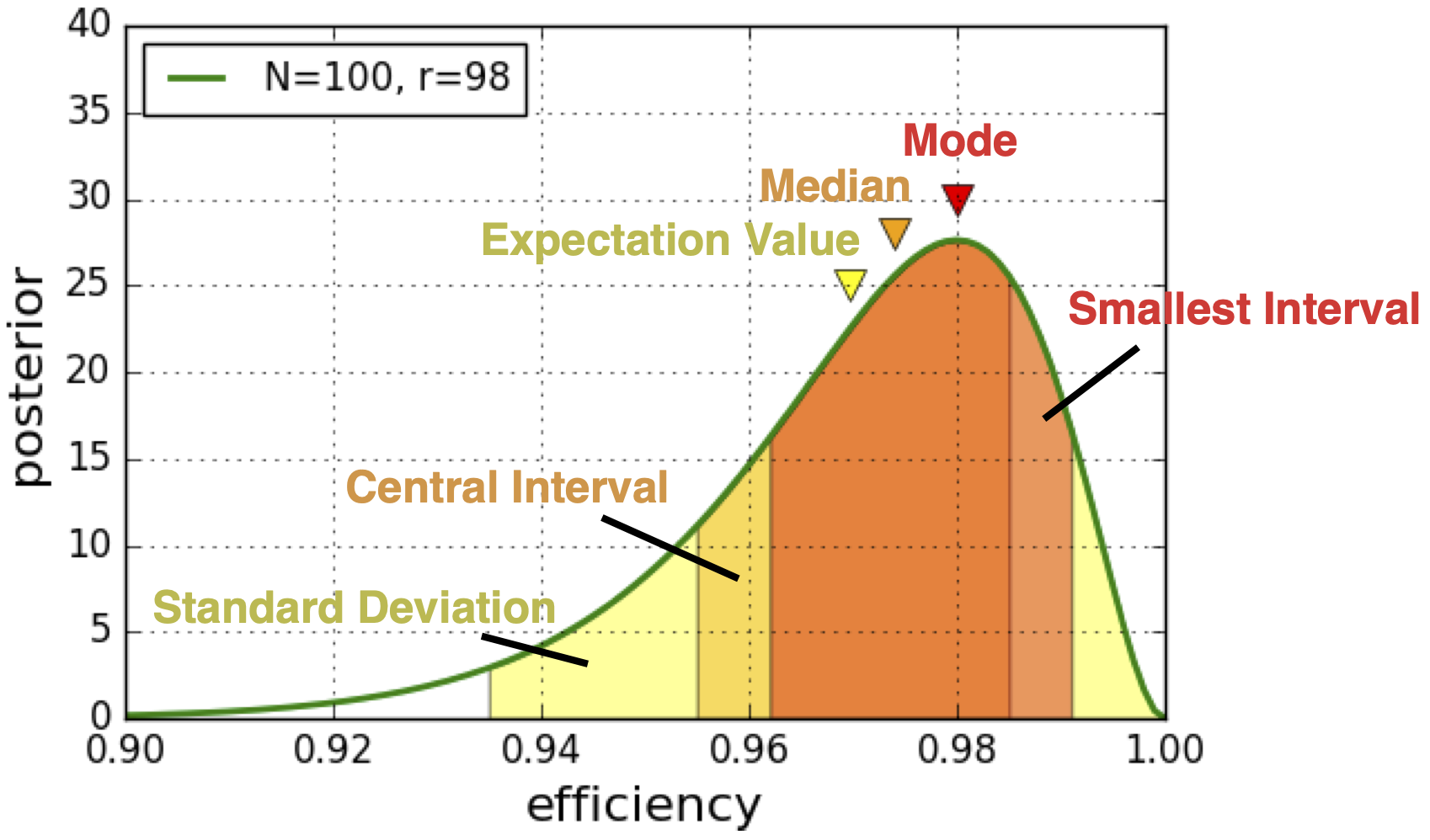
You can see that all three choices lead to different results. None of these is wrong or correct, it is just important to report exactly what point estimates you used and how you constructed your intervals. Here we could say for example that the most probable value (mode) of our posterior is 0.98 with a confidence interval of 0.962-0.991 (smallest interval including 68% of the probability density).

您會看到所有三個選擇導致不同的結果。 這些都不是錯誤或正確的，重要的是準確報告您使用的點估計以及間隔的構造方式。 在這里我們可以說，例如，我們后驗的最可能值(眾數)為0.98，置信區間為0.962-0.991(最小區間，包括68％的概率密度)。

結論 (Conclusions)

We performed a full Bayesian analysis starting by setting up a probability model, choosing appropriate priors all the way to summarizing the posterior with a point estimate and a corresponding interval. The advantage of the Bayesian approach is that we gain access to the full posterior probability distribution. This enabled us to elegantly incorporate prior knowledge, as for example the manufacturer's information, or a previous measurement. Furthermore, we saw that the choice of a wrong prior may have a significant influence on our results, highlighting that a careful choice of the prior and an evaluation of its consistency with the probability model and the posterior is of high importance in any Bayesian analysis.

我們從建立概率模型開始，進行了完整的貝葉斯分析，從一開始就選擇適當的先驗以總結出后驗點，并給出點估計和相應的間隔。 貝葉斯方法的優點是我們可以訪問全部后驗概率分布。 這使我們能夠優雅地結合先前的知識，例如制造商的信息或先前的測量。 此外，我們發現選擇錯誤的先驗可能會對我們的結果產生重大影響，強調在任何貝葉斯分析中，謹慎選擇先驗以及評估其與概率模型和后驗的一致性都非常重要。

A python notebook producing the numbers and figures can be found here.

可以在此處找到生成數字和數字的python筆記本。