In the last blog, we have learned how to create “Dynamic Maps Using ggplot2“. In this article, we will explore more into the 3D visualization in R programming language by using the plot3d package.

在上一個博客中，我們學習了如何創建“ 使用ggplot2使用動態地圖 ” 。 在本文中，我們將使用plot3d包對R編程語言中的3D可視化進行更多探索。

The plot3d package can be used to generate stunning 3-D plots in R. It can generate an interesting array of plots, but in this recipe, we will focus on creating 3-D scatterplots. These arise in situations where we have three variables, and we want to plot the triplets of values on the x–y–z space.

plot3d包可用于在R中生成令人驚嘆的3-D圖。它可以生成有趣的圖陣列，但是在本食譜中，我們將重點介紹創建3-D散點圖。 這些出現在我們有三個變量的情況下，我們想在x – y – z空間上繪制三元組值。

We will use a specific dataset to plot them into fancy plots using the plot3d package. The following steps are implemented to create 3D visualization in R.

我們將使用plot3d包使用特定的數據集將它們繪制成精美的圖。 執行以下步驟以在R中創建3D可視化 。

Step 1: Install the required packages which are needed for 3D visualization in R.

步驟1：在R中安裝3D可視化所需的必需軟件包。

> install.packages("rgl")
Installing package into ‘C:/Users/admin/Documents/R/win-library/3.6’
(as ‘lib’ is unspecified)
trying URL 'https://cran.rstudio.com/bin/windows/contrib/3.6/rgl_0.100.30.zip'
Content type 'application/zip' length 4253430 bytes (4.1 MB)
downloaded 4.1 MB
 
package ‘rgl’ successfully unpacked and MD5 sums checked
 
The downloaded binary packages are in
	C:\Users\admin\AppData\Local\Temp\Rtmpymt5Jd\downloaded_packages
> install.packages("plot3D")
Installing package into ‘C:/Users/admin/Documents/R/win-library/3.6’
(as ‘lib’ is unspecified)
package ‘plot3D’ successfully unpacked and MD5 sums checked
 
The downloaded binary packages are in
	C:\Users\admin\AppData\Local\Temp\Rtmpymt5Jd\downloaded_packages

Include the required libraries in the mentioned workspace.

在上述工作區中包括所需的庫。

> library(plot3D)
> library(rgl)

Step 2: We will use the dataset named “income.csv” which includes all the necessary parameters which are needed for understanding income rates of every employee.

步驟2：我們將使用名為“ income.csv ”的數據集，其中包括了解每個員工的收入率所需的所有必要參數。

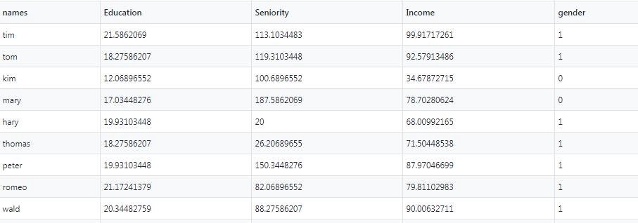
Step 3: Analyze the data structure of the dataset with the mentioned attributes.

步驟3：使用上述屬性分析數據集的數據結構。

> str(income)
'data.frame':	30 obs. of  5 variables:
 $ names    : Factor w/ 30 levels "brady","brandy",..: 27 29 14 17 10 26 22 24 30 18 ...
 $ Education: num  21.6 18.3 12.1 17 19.9 ...
 $ Seniority: num  113 119 101 188 20 ...
 $ Income   : num  99.9 92.6 34.7 78.7 68 ...
 $ gender   : int  1 1 0 0 1 1 1 1 1 1 ...

Step 4: It is important to understand the five-point summary of data before proceeding further. Visualization requires a lookout on bivariate and univariate analysis which is clearly understood with a five-point summary of data.

步驟4：在繼續進行之前，了解數據的五點摘要很重要。 可視化需要監視雙變量和單變量分析，并通過五點數據摘要清楚地了解。

> summary(income)
      names      Education       Seniority          Income     
 brady   : 1   Min.   :10.00   Min.   : 20.00   Min.   :17.61  
 brandy  : 1   1st Qu.:12.48   1st Qu.: 44.83   1st Qu.:36.39  
 brian   : 1   Median :17.03   Median : 94.48   Median :70.80  
 brittany: 1   Mean   :16.39   Mean   : 93.86   Mean   :62.74  
 bruce   : 1   3rd Qu.:19.93   3rd Qu.:133.28   3rd Qu.:85.93  
 charles : 1   Max.   :21.59   Max.   :187.59   Max.   :99.92  
 (Other) :24                                                   
     gender      
 Min.   :0.0000  
 1st Qu.:0.0000  
 Median :1.0000  
 Mean   :0.6333  
 3rd Qu.:1.0000  
 Max.   :1.0000

Step 5: Let us with bivariate analysis which focusses on 2-dimensional data and scatter plot is considered as an easy method to create the same.

步驟5：讓我們進行專注于二維數據的雙變量分析，而將散點圖視為創建該變量的簡便方法。

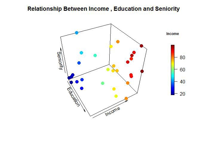
> scatter3D(x = inc$Education, y = inc$Income, z =inc$Seniority,
+           colvar = inc$Income,
+           pch = 16, cex = 1.5, xlab = "Education", ylab = "Income",
+           zlab = "Seniority", theta = 60, d = 2,clab = c("Income"),
+           colkey = list(length = 0.5, width = 0.5, cex.clab = 0.75,
+                         dist = -.08, side.clab = 3)
+           ,main = "Relationship Between Income , Education and Seniority")

Here, we are plotting “Education” in the x-axis, “Income” in the y-axis and the “Seniority” level in the z-axis. The distinct legends are created based on the range of income parameters. The plot is helpful to show the relationship between Income, Education, and Society.

在這里，我們在x軸上繪制“教育”，在y軸上繪制“收入”，在z軸上繪制“高級”水平。 根據收入參數范圍創建不同的圖例。 該圖有助于顯示收入，教育和社會之間的關系。

We can add more effects to the mentioned 3D plot with plane surfaces and ranges depicted in a specific order. Consider that we want to implement a linear regression model to establish the relationship between Seniority, Education and Income we can create a predictive model for the same.

我們可以使用特定順序描繪的平面和范圍為上述3D圖添加更多效果。 考慮到我們要實現線性回歸模型以建立資歷，教育和收入之間的關系，我們可以為此創建一個預測模型。

Step 6: Create a predictive model with the help of the RGL package. RGL is the 3D real-time rendering package in the R programming language. It provides high-level functions to create an interactive graph. To create a 3D plot of linear regression, we need to create a predictive model of the same.

步驟6：借助RGL軟件包創建預測模型。 RGL是R編程語言中的3D實時渲染包。 它提供了高級功能來創建交互式圖形。 要創建線性回歸的3D圖，我們需要創建相同的預測模型。

> lmin = lm(inc$Income~inc$Education+inc$Seniority)
> lmin
 
Call:
lm(formula = inc$Income ~ inc$Education + inc$Seniority)
 
Coefficients:
  (Intercept)  inc$Education  inc$Seniority  
     -50.0856         5.8956         0.1729  
> est = coef(lmin)
> a = est["inc$Education"]
> b = est["inc$Seniority"]
> c=-1
> d= est["(Intercept)"]
> est
  (Intercept) inc$Education inc$Seniority 
  -50.0856387     5.8955560     0.1728555 
> a
inc$Education 
     5.895556 
> b
inc$Seniority 
    0.1728555 
> c
[1] -1
> d
(Intercept) 
  -50.08564

Step 7: Once the required parameters for linear regression are taken into consideration, we can create an interactive graph where we plot the data points as a scattered graph and later embed the linear regression model in them.

步驟7：一旦考慮了線性回歸所需的參數，我們就可以創建一個交互式圖形，在其中將數據點繪制為散點圖，然后將線性回歸模型嵌入其中。

> plot3d(inc$Education,inc$Seniority,inc$Income, type = "s",
+        col = "blue", xlab = "Education",ylab = "Income",zlab =
+            "Seniority",box = FALSE)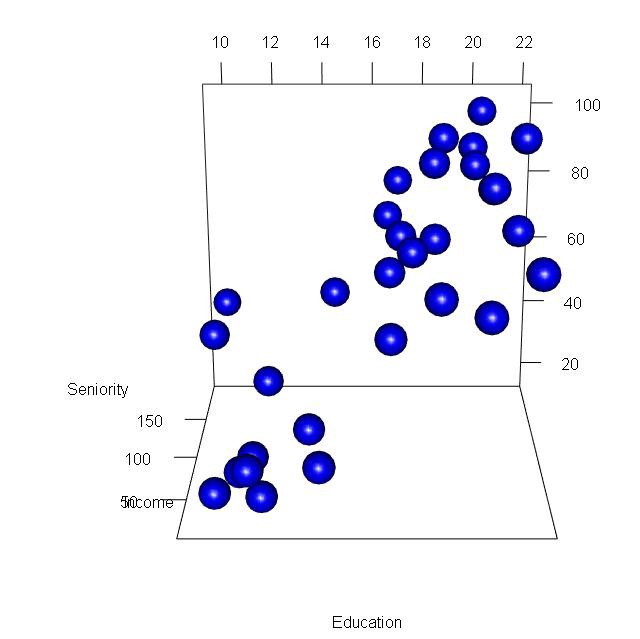

Now we will embed the linear regression line as mentioned below:

現在，我們將嵌入線性回歸線，如下所示：

planes3d(a,b,c,d, alpha = 0.5, col = "red")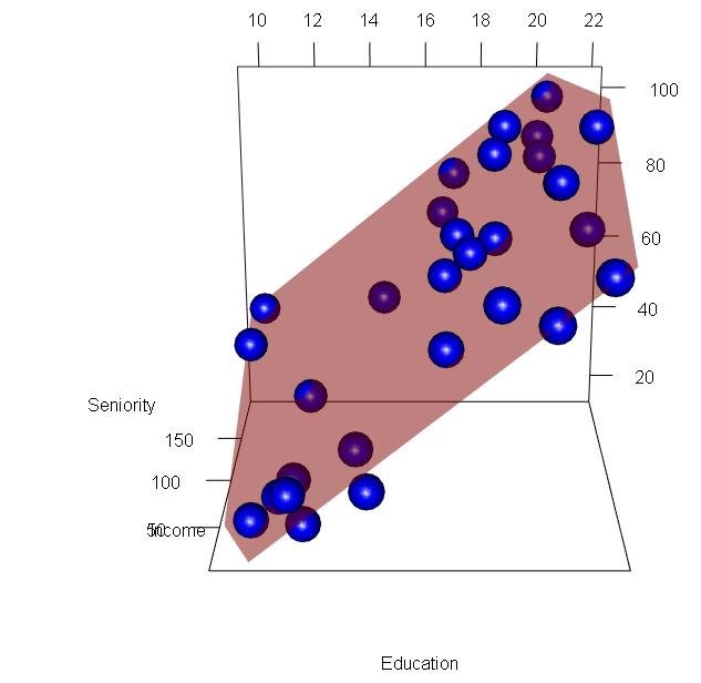

Step 8: We can create a surface plot that defines the volume and intensity of the data. Following steps are implemented to create a specific plot as mentioned below:

步驟8：我們可以創建一個表面圖來定義數據的數量和強度。 執行以下步驟來創建特定圖，如下所述：

> inc= read.csv("income2.csv")
> View(inc)
> row.names(inc)= inc$names
> inc
            names Education Seniority   Income gender
tim           tim  21.58621 113.10345 99.91717      1
tom           tom  18.27586 119.31034 92.57913      1
kim           kim  12.06897 100.68966 34.67873      0
mary         mary  17.03448 187.58621 78.70281      0
hary         hary  19.93103  20.00000 68.00992      1
thomas     thomas  18.27586  26.20690 71.50449      1
peter       peter  19.93103 150.34483 87.97047      1
romeo       romeo  21.17241  82.06897 79.81103      1
wald         wald  20.34483  88.27586 90.00633      1
matt         matt  10.00000 113.10345 45.65553      1
pam           pam  13.72414  51.03448 31.91381      0
pamela     pamela  18.68966 144.13793 96.28300      0
larry       larry  11.65517  20.00000 27.98250      1
karl         karl  16.62069  94.48276 66.60179      1
brian       brian  10.00000 187.58621 41.53199      1
dan           dan  20.34483  94.48276 89.00070      1
sim           sim  14.13793  20.00000 28.81630      0
kristin   kristin  16.62069  44.82759 57.68169      0
chiu         chiu  16.62069 175.17241 70.10510      1
bruce       bruce  20.34483 187.58621 98.83401      1
brady       brady  18.27586 100.68966 74.70470      1
brandy     brandy  14.55172 137.93103 53.53211      0
charles   charles  17.44828  94.48276 72.07892      1
timothy   timothy  10.41379  32.41379 18.57067      0
jerry       jerry  21.58621  20.00000 78.80578      1
garry       garry  11.24138  44.82759 21.38856      1
jena         jena  19.93103 168.96552 90.81404      0
ram           ram  11.65517  57.24138 22.63616      1
brittany brittany  12.06897  32.41379 17.61359      0
milly       milly  17.03448 106.89655 74.61096      0

Here, we convert the dataset into a separate vector and we also created the index based on the names of candidates. Text3d is the function that adds text to the plane surface. The text represents actual data representation. As we converted the row names with names of candidates, it becomes easy to display text in the 3D plot.

在這里，我們將數據集轉換為單獨的向量，并且還基于候選名稱創建了索引。 Text3d是將文本添加到平面的功能。 文本表示實際數據表示。 當我們用候選名稱轉換行名稱時，在3D圖中顯示文本變得很容易。

> text3D(x = inc$Education, y = inc$Income, z =inc$Seniority,
+        colvar = inc$Income,labels= row.names(inc),
+        pch = 16, cex = 0.8, xlab = "Education", ylab = "Income",
+        zlab = "Seniority", theta = 60, d = 2,clab = c("Income"),
+        colkey = list(length = 0.5, width = 0.5, cex.clab = 0.75,
+                      dist = -.08, side.clab = 3)
+        ,bty = "g")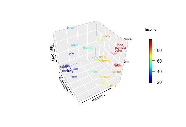

Step 9: We can convert the values in proper labels with distinct colors. This helps to visualize the 3D plot more easily and distinctly with a specific color range.

步驟9：我們可以將值轉換為具有不同顏色的適當標簽。 這有助于在特定顏色范圍內更輕松，更清晰地可視化3D圖。

> text3D(x = inc$Education, y = inc$Income, z =inc$Seniority,
+        colvar= inc$gender,col = c("red","black"),labels= row.names(inc),
+        pch = 16, cex = 0.8,xlab = "Education", ylab = "Income",
+        zlab = "Seniority", theta = 60, d = 2,clab = c("Income"),
+        bty = "g", colkey = FALSE)
> legend("topright", fill = c("red", "black"), legend=
+            c("Female","Male"), bty = "n")

等高線圖 (Contour Plots)

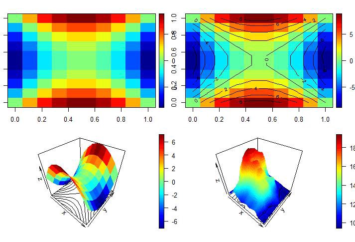
Contour plots visually represent the intensity of the plot. The color and graphical representation help in the visual analysis of data.

等高線圖直觀地表示了該圖的強度。 顏色和圖形表示有助于數據的可視化分析。

> x = y = seq(-3,3, length.out = 10)
> x
 [1] -3.0000000 -2.3333333 -1.6666667 -1.0000000 -0.3333333  0.3333333
 [7]  1.0000000  1.6666667  2.3333333  3.0000000
> y
 [1] -3.0000000 -2.3333333 -1.6666667 -1.0000000 -0.3333333  0.3333333
 [7]  1.0000000  1.6666667  2.3333333  3.0000000
> f = function(x,y){ z= (y^2-x^2)}
> m = outer(x,y,f)
> 
> image2D(m)
> image2D(m, contour = TRUE)
> 
> persp3D(z = m, contour = TRUE)
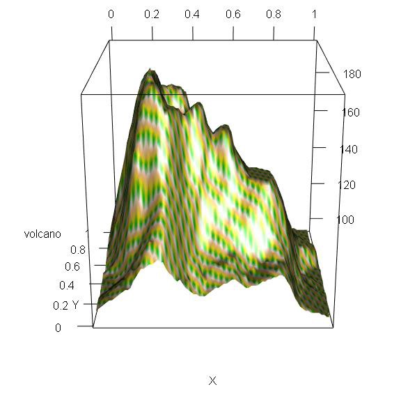
> persp3D(z = volcano, contour = TRUE)
> 
> library(rgl)
> c = terrain.colors(5)
> persp3d(z = volcano, contour = TRUE, col = c)

The output of the contour plot is mentioned below:

等高線圖的輸出如下所述：

The interactive 3d plot is mentioned below:

交互式3d圖如下所示：

We can also create a plot with an animation feature which increases the interactive rate. For this, it is important to install an “animation” package which helps in creating the plots as desired.

我們還可以創建帶有動畫功能的繪圖，以提高交互速率。 為此，重要的是安裝一個“動畫”程序包，該程序包可以幫助創建所需的繪圖。

> install.packages("plotrix")
Installing package into ‘C:/Users/admin/Documents/R/win-library/3.6’
(as ‘lib’ is unspecified)
trying URL 'https://cran.rstudio.com/bin/windows/contrib/3.6/plotrix_3.7-7.zip'
Content type 'application/zip' length 1132324 bytes (1.1 MB)
downloaded 1.1 MB
 
package ‘plotrix’ successfully unpacked and MD5 sums checked
 
The downloaded binary packages are in
	C:\Users\admin\AppData\Local\Temp\RtmpSCUS7b\downloaded_packages
> 
> install.packages("animation")
Installing package into ‘C:/Users/admin/Documents/R/win-library/3.6’
(as ‘lib’ is unspecified)
trying URL 'https://cran.rstudio.com/bin/windows/contrib/3.6/animation_2.6.zip'
Content type 'application/zip' length 548202 bytes (535 KB)
downloaded 535 KB
 
package ‘animation’ successfully unpacked and MD5 sums checked
 
The downloaded binary packages are in
	C:\Users\admin\AppData\Local\Temp\RtmpSCUS7b\downloaded_packages
> 
> library(plot3D)
> library(plotrix)
 
Attaching package: ‘plotrix’
 
The following object is masked from ‘package:rgl’:
 
    mtext3d
 
> library(animation)
> 
> x = y = seq(0,2*pi, length.out = 100)
> 
> z = mesh(x,y)
> u = z$x
> v = z$y
> 
> m= (sin(u)*sin(2*v)/2)
> n = (sin(2*u)*cos(v)*cos(v))
> o = (cos(2*u)*cos(v)*cos(v))
> 
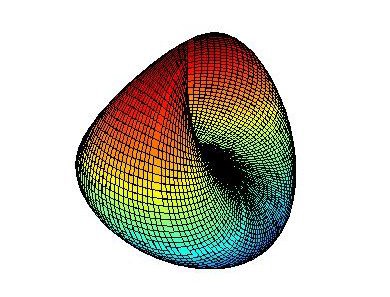
> surf3D(m, n,o, colvar = o, border = "black",colkey = FALSE,box = TRUE)
> 
> surf3D(m, n,o, colvar = o, border = "black",colkey = TRUE, box = TRUE,theta = 60)
> 
> surf3D(m, n,o, colvar = o, border = "black",colkey = TRUE,box = TRUE,theta = 100)
> 
> library("animation")
> saveHTML({
+     for (i in 1:100 ){
+         x = y = seq(0,2*pi, length.out = 100)
+         z = mesh(x,y)
+         u = z$x
+         v = z$y
+         m= (sin(u)*sin(2*v)/2)
+         n = (sin(2*u)*cos(v)*cos(v))
+         o = (cos(2*u)*cos(v)*cos(v))
+         surf3D(m, n,o, colvar = o, border = "black",colkey = FALSE,
+                theta = i, box = TRUE)
+     }
+ },interval = 0.1, ani.width = 500, ani.height = 1000)

The ranges of the graphs are depicted below:

圖的范圍如下所示：

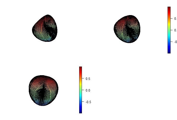
The file is saved with .html extension and represents the graphical animation of the values in three co-ordinates.

該文件以.html擴展名保存，并以三個坐標表示值的圖形動畫。

So, this was all about 3D visualization in R programming!

因此，這一切都與R編程中的3D可視化有關！

In the next section, we will be going to learn about Data Wrangling and Visualization in R programming language.

在下一節中，我們將學習R編程語言中的數據整理和可視化 。

Originally published https://blog.eduonix.com on March 27, 2020

最初 于 2020 年 3月27日發布 https://blog.eduonix.com