Pandas is a powerful package for data scientists. There are many reasons we use Pandas, e.g. Data wrangling, Data cleaning, and Data manipulation. Although, there is a method that rarely talks about regarding Pandas package and that is the Data plotting.

Pandas是數據科學家的強大工具包。 我們使用Pandas的原因很多，例如數據整理，數據清理和數據操作。 雖然，有一種方法很少談論有關Pandas軟件包的問題，??那就是Data plotting 。

Data plotting, just like the name implies, is a process to plot the data into some graph or chart to visualise the data. While we have much fancier visualisation package out there, some method is just available in the pandas plotting API.

顧名思義，數據繪制是將數據繪制到某些圖形或圖表中以可視化數據的過程。 雖然我們有很多更好的可視化程序包，但熊貓繪圖API中僅提供了一些方法。

Let’s see a few selected method I choose.

讓我們看看我選擇的一些選定方法。

1.拉德維茲 (1. radviz)

RadViz is a method to visualise N-dimensional data set into a 2D plot. The problem where we have more than 3-dimensional (features) data or more is that we could not visualise it, but RadViz allows it to happen.

RadViz是一種將N維數據集可視化為2D圖的方法。 我們擁有超過3維(特征)數據或更多數據的問題是我們無法可視化它，但是RadViz允許它發生。

According to Pandas, radviz allows us to project an N-dimensional data set into a 2D space where the influence of each dimension can be interpreted as a balance between the importance of all dimensions. In a simpler term, it means we could project a multi-dimensional data into a 2D space in a primitive way.

根據Pandas的說法，radviz允許我們將N維數據集投影到2D空間中，其中每個維的影響可以解釋為所有維的重要性之間的平衡。 簡單來說，這意味著我們可以以原始方式將多維數據投影到2D空間中 。

Let’s try to use the function in a sample dataset.

讓我們嘗試在樣本數據集中使用該函數。

#RadViz example
import pandas as pd
import seaborn as sns#To use the pd.plotting.radviz, you need a multidimensional data set with all numerical columns but one as the class column (should be categorical).mpg = sns.load_dataset('mpg')pd.plotting.radviz(mpg.drop(['name'], axis =1), 'origin')

Above is the result of RadViz function, but how you would interpret the plot?

上面是RadViz函數的結果，但是如何解釋該圖呢？

So, each Series in the DataFrame is represented as an evenly distributed slice on a circle. Just look at the example above, there is a circle with the series name.

因此，DataFrame中的每個Series均表示為圓上均勻分布的切片。 只要看一下上面的例子，就會有一個帶有系列名稱的圓圈。

Each data point then is plotted in the circle according to the value on each Series. Highly correlated Series in the DataFrame are placed closer on the unit circle. In the example, we could see the japan and europe car data are closer to the model_year while the usa car is closer to the displacement. It means japan and europe car are most likely correlated to the model_year while usa car is with the displacement.

然后，根據每個系列的值將每個數據點繪制在圓圈中。 DataFrame中高度相關的Series位于單位圓上。 在示例中，我們可以看到日本和歐洲的汽車數據更接近model_year，而美國汽車的數據更接近排量。 這意味著日本和歐洲的汽車最有可能與model_year相關，而美國汽車則與排量相關。

If you want to know more about RadViz, you could check the paper here.

如果您想了解有關RadViz的更多信息，可以在此處查看該論文。

2. bootstrap_plot (2. bootstrap_plot)

According to Pandas, the bootstrap plot is used to estimate the uncertainty of a statistic by relying on random sampling with replacement. In simpler words, it is used to trying to determine the uncertainty in fundamental statistic such as mean and median by resampling the data with replacement (you could sample the same data multiple times). You could read more about bootstrap here.

根據Pandas的說法， 引導程序圖依賴于隨機抽樣和替換來估計統計的不確定性。 用簡單的話來說， 它用于嘗試通過替換對數據進行重采樣來確定基本統計數據的不確定性，例如均值和中位數 (您可以多次采樣同一數據)。 您可以在此處閱讀有關引導的更多信息。

The boostrap_plot function will generate bootstrapping plots for mean, median and mid-range statistics for the given number of samples of the given size. Let’s try using the function with an example dataset.

boostrap_plot函數將為給定大小的給定數量的樣本生成均值，中值和中間范圍統計量的自舉圖。 讓我們嘗試將函數與示例數據集一起使用。

For example, I have the mpg dataset and already have the information regarding the mpg feature data.

例如，我有mpg數據集，并且已經有了有關mpg特征數據的信息。

mpg['mpg'].describe()

We could see that the mpg mean is 23.51 and the median is 23. Although this is just a snapshot of the real-world data. How are the values actually is in the population is unknown, that is why we could measure the uncertainty with the bootstrap methods.

我們可以看到mpg平均值為23.51，中位數為23。盡管這只是真實數據的快照。 實際值如何在總體中是未知的，這就是為什么我們可以使用自舉法來測量不確定性的原因。

#bootstrap_plot examplepd.plotting.bootstrap_plot(mpg['mpg'],size = 50 , samples = 500)

Above is the result example of bootstap_plot function. Mind that the result could be different than the example because it relies on random resampling.

上面是bootstap_plot函數的結果示例。 請注意，結果可能與示例不同，因為它依賴于隨機重采樣。

We could see in the first set of the plots (first row) is the sampling result, where the x-axis is the repetition, and the y-axis is the statistic. In the second set is the statistic distribution plot (Mean, Median and Midrange).

我們可以在第一組圖(第一行)中看到采樣結果，其中x軸是重復項，y軸是統計量。 第二組是統計分布圖(均值，中位數和中位數)。

Take an example of the mean, most of the result is around 23, but it could be between 22.5 and 25 (more or less). This set the uncertainty in the real world that the mean in the population could be between 22.5 and 25. Note that there is a way to estimate the uncertainty by taking the values in the position 2.5% and 97.5% quantile (95% confident) although it is still up to your judgement.

以平均值為例，大多數結果在23左右，但可能在22.5到25之間(或多或少)。 這設置了現實世界中的不確定性，即總體平均值可能在22.5和25之間。請注意，盡管有2.5％和97.5％的分位數(95％的置信度)，但是有一種方法可以估計不確定性這仍然取決于您的判斷。

3. lag_plot (3. lag_plot)

A lag plot is a scatter plot for a time series and the same data lagged. Lag itself is a fixed amount of passing time; for example, lag 1 is a day 1 (Y1) with a 1-day time lag (Y1+1 or Y2).

滯后圖是時間序列的散點圖，并且相同數據滯后。 滯后本身是固定的通過時間； 例如，滯后1是第1天(Y1)，時滯為1天(Y1 + 1或Y2)。

A lag plot is used to checks whether the time series data is random or not, and if the data is correlated with themselves. Random data should not have any identifiable patterns, such as linear. Although, why we bother with randomness or correlation? This is because many Time Series models are based on the linear regression, and one assumption is no correlation (Specifically is no Autocorrelation).

滯后圖用于檢查時間序列數據是否隨機，以及數據是否與自身相關。 隨機數據不應具有任何可識別的模式，例如線性。 雖然，為什么我們要擾亂隨機性或相關性？ 這是因為許多時間序列模型都基于線性回歸，并且一個假設是不相關的(特別是沒有自相關)。

Let’s try with an example data. In this case, I would use a specific package to scrap stock data from Yahoo Finance called yahoo_historical.

讓我們嘗試一個示例數據。 在這種情況下，我將使用一個名為yahoo_historical的特定程序包從Yahoo Finance抓取股票數據。

pip install yahoo_historical

With this package, we could scrap a specific stock data history. Let’s try it.

有了這個軟件包，我們可以抓取特定的庫存數據歷史記錄。 讓我們嘗試一下。

from yahoo_historical import Fetcher#We would scrap the Apple stock data. I would take the data between 1 January 2007 to 1 January 2017 
data = Fetcher("AAPL", [2007,1,1], [2017,1,1])
apple_df = data.getHistorical()#Set the date as the index
apple_df['Date'] = pd.to_datetime(apple_df['Date'])
apple_df = apple_df.set_index('Date')

Above is our Apple stock dataset with the date as the index. We could try to plot the data to see the pattern over time with a simple method.

上面是我們的Apple股票數據集，其中以日期為索引。 我們可以嘗試使用一種簡單的方法來繪制數據以查看隨時間變化的模式。

apple_df['Adj Close'].plot()

We can see the Adj Close is increasing over time but is the data itself shown any pattern in with their lag? In this case, we would use the lag_plot.

我們可以看到，隨著時間的推移，“關閉收盤價”(Adj Close)不斷增加，但是數據本身是否顯示出任何與滯后有關的模式？ 在這種情況下，我們將使用lag_plot。

#Try lag 1 day
pd.plotting.lag_plot(apple_df['Adj Close'], lag = 1)

As we can see in the plot above, it is almost near linear. It means there is a correlation between daily Adj Close. It is expected as the daily price of the stock would not be varied much in each day.

如上圖所示，它幾乎接近線性。 這意味著每日調整關閉之間存在相關性。 可以預期，因為股票的每日價格每天不會有太大變化。

How about a weekly basis? Let’s try to plot it

每周一次如何？ 讓我們嘗試繪制它

#The data only consist of work days, so one week is 5 dayspd.plotting.lag_plot(apple_df['Adj Close'], lag = 5)

We can see the pattern is similar to the lag 1 plot. How about 365 days? would it have any differences?

我們可以看到該模式類似于滯后1圖。 365天怎么樣？ 有什么區別嗎？

pd.plotting.lag_plot(apple_df['Adj Close'], lag = 365)

We can see right now the pattern becomes more random, although the non-linear pattern still exists.

現在我們可以看到模式變得更加隨機，盡管非線性模式仍然存在。

4. scatter_matrix (4. scatter_matrix)

The scatter_matrix is just like the name implies; it creates a matrix of scatter plot. Let’s try it with an example at once.

顧名思義， scatter_matrix就是一樣。 它創建了散點圖矩陣。 讓我們立即嘗試一個示例。

import matplotlib.pyplot as plttips = sns.load_dataset('tips')
pd.plotting.scatter_matrix(tips, figsize = (8,8))
plt.show()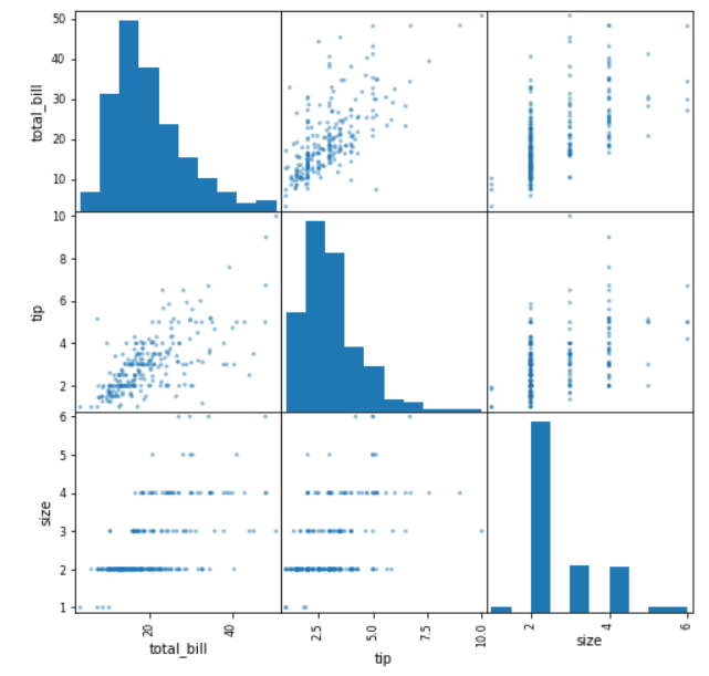

We can see the scatter_matrix function automatically detects the numerical features within the Data Frame we passed to the function and create a matrix of the scatter plot.

我們可以看到scatter_matrix函數自動檢測我們傳遞給該函數的數據框內的數字特征，并創建散點圖的矩陣。

In the example above, between two numerical features are plotted together to create a scatter plot (total_bill and size, total_bill and tip, and tip and size). Whereas, the diagonal part is the histogram of the numerical features.

在上面的示例中，兩個數字特征之間被繪制在一起以創建散點圖(total_bill和size，total_bill和tip，以及tip和size)。 而對角線部分是數值特征的直方圖。

This is a simple function but powerful enough as we could get much information with a single line of code.

這是一個簡單的功能，但功能足夠強大，因為我們可以用一行代碼來獲取很多信息。

結論 (Conclusion)

Here I have shown you 4 different pandas plotting functions that you should know, that includes:

在這里，我向您展示了您應該了解的4種不同的熊貓繪圖功能，其中包括：

1. radviz
   拉德維茲
2. bootstrap_plot
   bootstrap_plot
3. lag_plot
   lag_plot
4. scatter_matrix
   scatter_matrix

I hope it helps!

希望對您有所幫助！