官網API

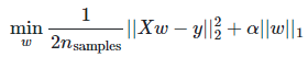
一、線性回歸

針對的是損失函數loss faction

Ⅰ、Lasso Regression

采用L1正則，會使得w值整體偏小；w會變小從而達到降維的目的
在這里插入圖片描述

import numpy as np
from sklearn.linear_model import Lasso
from sklearn.linear_model import SGDRegressorX = 2 * np.random.rand(100, 1)
y = 4 + 3 * X + np.random.randn(100, 1)lasso_reg = Lasso(alpha=0.15, max_iter=10000)
lasso_reg.fit(X, y)
print("w0=",lasso_reg.intercept_)
print("w1=",lasso_reg.coef_)sgd_reg = SGDRegressor(penalty='l1', max_iter=10000)
sgd_reg.fit(X, y.ravel())
print("w0=",sgd_reg.intercept_)
print("w1=",lasso_reg.coef_)

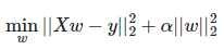
Ⅱ、Ridge Regression（嶺回歸）

采用L2正則，會使得有的w趨近1，有的w趨近0；當w趨近于0的時候，相對于可以忽略，w會變少也可以達到降維的目的（深度學習模型建立首選）
在這里插入圖片描述

import numpy as np
from sklearn.linear_model import Ridge
from sklearn.linear_model import SGDRegressor#隨機梯度下降回歸#模擬數據
X = 2 * np.random.rand(100,1)
y = 4 + 3 * X + np.random.randn(100,1)ridge_reg = Ridge(alpha=1,solver='auto')#創建一個ridge回歸模型實例，alpha為懲罰項前的系數
ridge_reg.fit(X,y)
print("w0=",ridge_reg.intercept_)#w0
print("w1=",ridge_reg.coef_)#w1sgd_reg = SGDRegressor(penalty='l2')
sgd_reg.fit(X,y.ravel())
print("w0=",sgd_reg.intercept_)#w0
print("w1=",sgd_reg.coef_)#w1

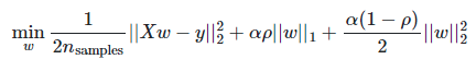
Ⅲ、Elastic Net回歸

當你不清楚使用L1正則化還是L2正則化的時候，可以采用Elastic Net
在這里插入圖片描述

import numpy as np
from sklearn.linear_model import ElasticNet
from sklearn.linear_model import SGDRegressorX = 2 * np.random.rand(100, 1)
y = 4 + 3 * X + np.random.randn(100, 1)elastic_net = ElasticNet(alpha=0.0001, l1_ratio=0.15)
elastic_net.fit(X, y)
#print(elastic_net.predict(1.5))
print("w0=",elastic_net.intercept_)
print("w1=",elastic_net.coef_)sgd_reg = SGDRegressor(penalty='elasticnet', max_iter=1000)
sgd_reg.fit(X, y.ravel())
#print(sgd_reg.predict(1.5))
print("w0=",sgd_reg.intercept_)
print("w1=",sgd_reg.coef_)

Ⅳ、總結

①算法選擇順序，Ridge Regression (L2正則化) --> ElasticNet (即包含L1又包含L2) --> Lasso Regression (L1正則化)

②正則化L1和L2有什么區別？

答：L1是w絕對值加和，L2是w平方加和。L1的有趣的現象是會使得w有的接近于0，有的接近于1，
L1更多的會用在降維上面，因為有的是0有的是1，我們也稱之為稀疏編碼。
L2是更常用的正則化手段，它會使得w整體變小

超參數alpha 在Rideg類里面就直接是L2正則的權重
超參數alpha 在Lasso類里面就直接是L1正則的權重
超參數alpha 在ElasticNet和SGDRegressor里面是損失函數里面的alpha
超參數l1_ration 在ElasticNet和SGDRegressor里面是損失函數的p

二、多項式回歸

針對的是數據預處理進行特征處理，跟歸一化一樣，都是針對的是數據
多項式回歸其實是線性回歸的一種拓展。
多項式回歸：叫回歸但并不是去做擬合的算法
PolynomialFeatures是來做預處理的，來轉換我們的數據，把數據進行升維！

import numpy as np
import matplotlib.pyplot as plt
from sklearn.preprocessing import PolynomialFeatures
from sklearn.linear_model import LinearRegression

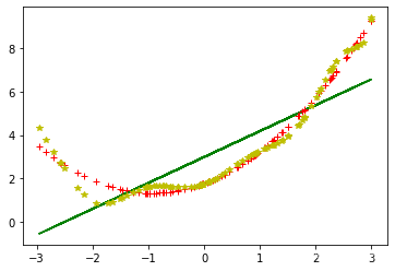
m = 100#100個樣本
X = 6 * np.random.rand(m, 1) - 3#m行1列的數，數的取值范圍在[-3,3]
y = 0.5 * X ** 2 + X + 2 + np.random.randn(m, 1)plt.plot(X, y, 'b.')

在這里插入圖片描述

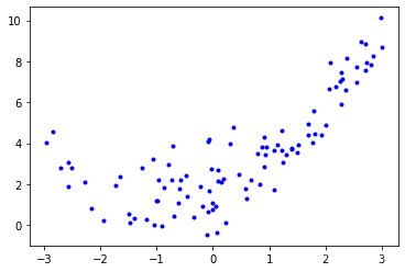
d = {1: 'g-', 2: 'r+', 10: 'y*'}
for i in d:poly_features = PolynomialFeatures(degree=i, include_bias=False)#degree超參數可以改變，當然若太大會出現過擬合現象，導致效果更加糟糕X_poly = poly_features.fit_transform(X)print(X[0])print(X_poly[0])print(X_poly[:, 0])lin_reg = LinearRegression(fit_intercept=True)lin_reg.fit(X_poly, y)print(lin_reg.intercept_, lin_reg.coef_)y_predict = lin_reg.predict(X_poly)plt.plot(X_poly[:, 0], y_predict, d[i])plt.show()
"""
[-1.17608282]
[-1.17608282]
[-1.17608282  0.84008756 -0.47456115  1.09332609 -0.08048591  2.56227793-2.16089094  2.9934595  -0.97719578 -0.35093548 -0.01833382 -2.578095490.90594767  1.23236141  0.5809494  -1.03761487  1.07926559 -1.015365042.08713351  1.68679419  0.36108667  0.0739686  -0.60676473 -0.09778250.93322126 -0.98029008  1.80329174 -2.7079627   2.27067075 -0.23098381-2.84414673  2.80368239  1.13965085  0.60386564  1.5068452   0.084835792.54605719  2.25506764 -0.57412233  1.40321778  0.08664762  1.79293147-0.72311264 -1.39573162  0.15066435 -2.56825076  1.6992054   0.306551442.27792527  0.05690445  1.91725839  2.70744724 -0.46459041  1.24513038-0.90932212  2.71793477 -1.64319111  1.49955188  2.17534115 -2.505103912.72835224 -0.17797949 -0.07305404 -0.60531858  0.90754969  0.1864542.63700818  2.00439925 -1.26906332 -0.03326623  0.95249887  2.988010311.39131364 -1.46984234  0.67347918  1.30899516 -0.68746311 -0.078952172.847029   -1.94670177 -0.73970148 -1.05884194 -2.95987324 -2.27319748-0.01555128 -0.86999284  0.45600536  1.21528784 -1.72581767  0.22440468-1.50353748  2.36782931  2.30633509  1.76346603 -0.79567338 -0.061536510.87272525  0.78535366  2.36179793  2.05667417]
[2.99104579] [[1.19669575]]
[-1.17608282]
[-1.17608282  1.38317079]
[-1.17608282  0.84008756 -0.47456115  1.09332609 -0.08048591  2.56227793-2.16089094  2.9934595  -0.97719578 -0.35093548 -0.01833382 -2.578095490.90594767  1.23236141  0.5809494  -1.03761487  1.07926559 -1.015365042.08713351  1.68679419  0.36108667  0.0739686  -0.60676473 -0.09778250.93322126 -0.98029008  1.80329174 -2.7079627   2.27067075 -0.23098381-2.84414673  2.80368239  1.13965085  0.60386564  1.5068452   0.084835792.54605719  2.25506764 -0.57412233  1.40321778  0.08664762  1.79293147-0.72311264 -1.39573162  0.15066435 -2.56825076  1.6992054   0.306551442.27792527  0.05690445  1.91725839  2.70744724 -0.46459041  1.24513038-0.90932212  2.71793477 -1.64319111  1.49955188  2.17534115 -2.505103912.72835224 -0.17797949 -0.07305404 -0.60531858  0.90754969  0.1864542.63700818  2.00439925 -1.26906332 -0.03326623  0.95249887  2.988010311.39131364 -1.46984234  0.67347918  1.30899516 -0.68746311 -0.078952172.847029   -1.94670177 -0.73970148 -1.05884194 -2.95987324 -2.27319748-0.01555128 -0.86999284  0.45600536  1.21528784 -1.72581767  0.22440468-1.50353748  2.36782931  2.30633509  1.76346603 -0.79567338 -0.061536510.87272525  0.78535366  2.36179793  2.05667417]
[1.77398327] [[0.96156952 0.516698  ]]
[-1.17608282]
[-1.17608282  1.38317079 -1.6267234   1.91316143 -2.25003628  2.64622901-3.11218446  3.66018667 -4.30468264  5.06266328]
[-1.17608282  0.84008756 -0.47456115  1.09332609 -0.08048591  2.56227793-2.16089094  2.9934595  -0.97719578 -0.35093548 -0.01833382 -2.578095490.90594767  1.23236141  0.5809494  -1.03761487  1.07926559 -1.015365042.08713351  1.68679419  0.36108667  0.0739686  -0.60676473 -0.09778250.93322126 -0.98029008  1.80329174 -2.7079627   2.27067075 -0.23098381-2.84414673  2.80368239  1.13965085  0.60386564  1.5068452   0.084835792.54605719  2.25506764 -0.57412233  1.40321778  0.08664762  1.79293147-0.72311264 -1.39573162  0.15066435 -2.56825076  1.6992054   0.306551442.27792527  0.05690445  1.91725839  2.70744724 -0.46459041  1.24513038-0.90932212  2.71793477 -1.64319111  1.49955188  2.17534115 -2.505103912.72835224 -0.17797949 -0.07305404 -0.60531858  0.90754969  0.1864542.63700818  2.00439925 -1.26906332 -0.03326623  0.95249887  2.988010311.39131364 -1.46984234  0.67347918  1.30899516 -0.68746311 -0.078952172.847029   -1.94670177 -0.73970148 -1.05884194 -2.95987324 -2.27319748-0.01555128 -0.86999284  0.45600536  1.21528784 -1.72581767  0.22440468-1.50353748  2.36782931  2.30633509  1.76346603 -0.79567338 -0.061536510.87272525  0.78535366  2.36179793  2.05667417]
[1.75155522] [[ 0.96659081  1.47322289 -0.32379381 -1.09309828  0.22053653  0.3517641-0.03986542 -0.04423885  0.00212836  0.00193739]]
"""

在這里插入圖片描述

完整代碼如下：

import numpy as np
import matplotlib.pyplot as plt
from sklearn.preprocessing import PolynomialFeatures
from sklearn.linear_model import LinearRegressionm = 100#100個樣本
X = 6 * np.random.rand(m, 1) - 3#m行1列的數，m = 100#100個樣本
X = 6 * np.random.rand(m, 1) - 3#m行1列的數，數的取值范圍在[-3,3]
y = 0.5 * X ** 2 + X + 2 + np.random.randn(m, 1)plt.plot(X, y, 'b.')#數的取值范圍在[-3,3]
y = 0.5 * X ** 2 + X + 2 + np.random.randn(m, 1)plt.plot(X, y, 'b.')d = {1: 'g-', 2: 'r+', 10: 'y*'}
for i in d:poly_features = PolynomialFeatures(degree=i, include_bias=False)X_poly = poly_features.fit_transform(X)print(X[0])print(X_poly[0])print(X_poly[:, 0])lin_reg = LinearRegression(fit_intercept=True)lin_reg.fit(X_poly, y)print(lin_reg.intercept_, lin_reg.coef_)y_predict = lin_reg.predict(X_poly)plt.plot(X_poly[:, 0], y_predict, d[i])plt.show()

三、案例實戰

保險公司的一份數據集，里面含有多人的age、sex、bmi、children、smoker、region、charges。
年齡、性別、BMI肥胖指數、有幾個孩子、是否吸煙、居住區域、醫療開銷。
很顯然，這是個有監督的學習，保險公司肯定是想通過其他因素來確定處某個人的醫療開銷，來一個人，我可以通過他的年齡、性別、BMI肥胖指數、有幾個孩子、是否吸煙、居住區域來推測出這個人的醫療開銷。
故，這里的y為charges，各因素為age、sex、bmi、children、smoker、region。
在這里插入圖片描述

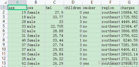
免費保險公司用戶信息數據集下載，這里采用的是CSV文件，也就是數據之間通過逗號隔開的數據集。
逗號分隔值（Comma-Separated Values，CSV，有時也稱為字符分隔值，因為分隔字符也可以不是逗號）

import pandas as pd
import matplotlib.pyplot as plt
from sklearn.preprocessing import PolynomialFeatures
from sklearn.linear_model import LinearRegression

data = pd.read_csv('./insurance.csv')#該路徑為數據集的路徑
print(type(data))
print(data.head())#輸出前5條數據
print(data.tail())#輸出后5條數據
# describe做簡單的統計摘要
print(data.describe())
"""
<class 'pandas.core.frame.DataFrame'>age     sex     bmi  children smoker     region      charges
0   19  female  27.900         0    yes  southwest  16884.92400
1   18    male  33.770         1     no  southeast   1725.55230
2   28    male  33.000         3     no  southeast   4449.46200
3   33    male  22.705         0     no  northwest  21984.47061
4   32    male  28.880         0     no  northwest   3866.85520age     sex    bmi  children smoker     region     charges
1333   50    male  30.97         3     no  northwest  10600.5483
1334   18  female  31.92         0     no  northeast   2205.9808
1335   18  female  36.85         0     no  southeast   1629.8335
1336   21  female  25.80         0     no  southwest   2007.9450
1337   61  female  29.07         0    yes  northwest  29141.3603age          bmi     children       charges
count  1338.000000  1338.000000  1338.000000   1338.000000
mean     39.207025    30.663397     1.094918  13270.422265
std      14.049960     6.098187     1.205493  12110.011237
min      18.000000    15.960000     0.000000   1121.873900
25%      27.000000    26.296250     0.000000   4740.287150
50%      39.000000    30.400000     1.000000   9382.033000
75%      51.000000    34.693750     2.000000  16639.912515
max      64.000000    53.130000     5.000000  63770.428010
"""

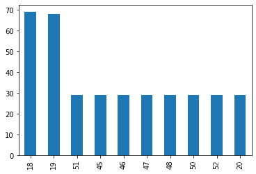
# 采樣要均勻
data_count = data['age'].value_counts()#看看age有多少個不同的年齡，各個年齡的人一共有幾個人
print(data_count)
data_count[:10].plot(kind='bar')#將年齡的前10個進行柱狀圖展示
plt.show()
# plt.savefig('./temp')#可以指定將圖進行保存的路徑
"""
18    69
19    68
51    29
45    29
46    29
47    29
48    29
50    29
52    29
20    29
26    28
54    28
53    28
25    28
24    28
49    28
23    28
22    28
21    28
27    28
28    28
31    27
29    27
30    27
41    27
43    27
44    27
40    27
42    27
57    26
34    26
33    26
32    26
56    26
55    26
59    25
58    25
39    25
38    25
35    25
36    25
37    25
63    23
60    23
61    23
62    23
64    22
Name: age, dtype: int64
"""

在這里插入圖片描述

print(data.corr())
"""age       bmi  children   charges
age       1.000000  0.109272  0.042469  0.299008
bmi       0.109272  1.000000  0.012759  0.198341
children  0.042469  0.012759  1.000000  0.067998
charges   0.299008  0.198341  0.067998  1.000000
"""

reg = LinearRegression()
x = data[['age', 'sex', 'bmi', 'children', 'smoker', 'region']]
y = data['charges']
# python3.6 報錯 sklearn ValueError: could not convert string to float: 'northwest'，加入一下幾行解決
x = x.apply(pd.to_numeric, errors='coerce')#有的數據集類型是字符串，需要通過to_numeric方法轉換為數值型
y = y.apply(pd.to_numeric, errors='coerce')
x.fillna(0, inplace=True)#數據集中為空的地方填充為0
y.fillna(0, inplace=True)poly_features = PolynomialFeatures(degree=3, include_bias=False)
X_poly = poly_features.fit_transform(x)reg.fit(X_poly, y)
print("w0=",reg.intercept_)#w0
print("w1=",reg.coef_)#w1
"""
w0= 14959.173791946276
w1= [ 5.86755877e+02 -8.66943361e-09 -2.43090741e+03  2.46877353e+03-2.34731345e-09  6.66457112e-10 -1.20823237e+01  2.22654961e-096.99860524e+00 -1.94583589e+02 -2.67144085e-10  4.64133620e-107.31601446e-11  3.21392690e-10 -1.89132265e-10  7.45785655e-113.91901267e-09  9.19625484e+01 -1.49720497e+02  0.00000000e+000.00000000e+00  2.76208814e+03  0.00000000e+00  0.00000000e+000.00000000e+00  0.00000000e+00  0.00000000e+00  9.96980980e-020.00000000e+00  4.50579510e-02  3.12743917e+00  0.00000000e+000.00000000e+00  0.00000000e+00  0.00000000e+00  0.00000000e+000.00000000e+00  0.00000000e+00 -2.30842696e-01 -1.20554724e+000.00000000e+00  0.00000000e+00 -4.28257797e+00  0.00000000e+000.00000000e+00  0.00000000e+00  0.00000000e+00  0.00000000e+000.00000000e+00  0.00000000e+00  0.00000000e+00  0.00000000e+000.00000000e+00  0.00000000e+00  0.00000000e+00  0.00000000e+000.00000000e+00  0.00000000e+00  0.00000000e+00  0.00000000e+000.00000000e+00  0.00000000e+00  0.00000000e+00 -9.34651320e-015.89748395e+00  0.00000000e+00  0.00000000e+00 -5.02728643e+010.00000000e+00  0.00000000e+00  0.00000000e+00  0.00000000e+000.00000000e+00 -2.25687557e+02  0.00000000e+00  0.00000000e+000.00000000e+00  0.00000000e+00  0.00000000e+00  0.00000000e+000.00000000e+00  0.00000000e+00  0.00000000e+00]
"""

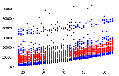
y_predict = reg.predict(X_poly)plt.plot(x['age'], y, 'b.')
plt.plot(X_poly[:, 0], y_predict, 'r.')
plt.show()

在這里插入圖片描述

完整代碼如下：

import pandas as pd
import matplotlib.pyplot as plt
from sklearn.preprocessing import PolynomialFeatures
from sklearn.linear_model import LinearRegressiondata = pd.read_csv('./insurance.csv')
print(type(data))
print(data.head())#輸出前5條數據
print(data.tail())#輸出后5條數據
# describe做簡單的統計摘要
print(data.describe())# 采樣要均勻
data_count = data['age'].value_counts()#看看age有多少個不同的年齡，各個年齡的人一共有幾個人
print(data_count)
data_count[:10].plot(kind='bar')#將年齡的前10個進行柱狀圖展示
plt.show()
# plt.savefig('./temp')#將圖進行保存print(data.corr())#輸出列和列之間的相關性reg = LinearRegression()
x = data[['age', 'sex', 'bmi', 'children', 'smoker', 'region']]
y = data['charges']
# python3.6 報錯 sklearn ValueError: could not convert string to float: 'northwest'，加入一下幾行解決
x = x.apply(pd.to_numeric, errors='coerce')
y = y.apply(pd.to_numeric, errors='coerce')
x.fillna(0, inplace=True)
y.fillna(0, inplace=True)poly_features = PolynomialFeatures(degree=3, include_bias=False)
X_poly = poly_features.fit_transform(x)reg.fit(X_poly, y)
print(reg.coef_)
print(reg.intercept_)y_predict = reg.predict(X_poly)plt.plot(x['age'], y, 'b.')
plt.plot(X_poly[:, 0], y_predict, 'r.')
plt.show()

四、總結

Ⅰ多項式回歸：叫回歸但并不是去做擬合的算法，PolynomialFeatures是來做預處理的，來轉換我們的數據，把數據進行升維！

Ⅱ升維有什么用？

答：升維就是增加更多的影響Y結果的因素，這樣考慮的更全面，最終的目的是要增加準確率！
還有時候，就像PolynomialFeatures去做升維，是為了讓線性模型去擬合非線性的數據！

ⅢPolynomialFeatures是怎么升維的？

答：可以傳入degree超參數，如果等于2，那么就會在原有維度基礎之上增加二階的數據變化！更高階的以此類推

Ⅳ如果數據是非線性的變化，但是就想用線性的模型去擬合這個非線性的數據，怎么辦？

答：1，非線性的數據去找非線性的算法生成的模型去擬合
2，可以把非線性的數據進行變化，變成類似線性的變化，然后使用線性的模型去擬合
PolynomialFeatures類其實就是這里說的第二種方式

Ⅴ保險的案例：

目的：未來來個新的人，可以通過模型來預測他的醫療花銷，所以，就把charges列作為y，其他列作為X維度

Ⅵ為什么每行沒有人名？

答：人名不會對最終的Y結果產生影響，所以可以不用

Ⅶ為什么要觀測注意數據多樣性，采樣要均勻？

答：就是因為你要的模型的功能是對任何年齡段的人都有一個好的預測，那么你的模型在訓練的時候讀取的數據集，就得包含各個年齡段的數據，而且各個年齡段也得數據均勻，防止過擬合！

Ⅷ什么是Pearson相關系數？

答：Pearson相關系數是來測量兩組變量之間的線性相關性的！Pearson相關系數的區間范圍是-1到1之間
如果越接近于-1，說明兩組變量越負相關，一個變大，另一個變小，反之如果越接近于1，說明兩組變量越正相關，一個變大，另一個也跟著變大，如果越接近于0，說明越不相關，即一個變大或變小，另一個沒什么影響！
通過Pearson相關系數，如果發現兩個維度之間，相關系數接近于1，可以把其中一個去掉，做到降維！
通過Pearson相關系數，如果發現某個維度和結果Y之間的相關系數接近于0，可以把這個維度去掉，降維！